Azimuthal Integration (in Pyxem!)

pyxem now includes built in azimuthal integration functionality. This is useful for extracting radial profiles from diffraction patterns in 1 or 2 dimensions. The new method will split the pixels into radial bins and then sum the intensity in each bin resulting in a Diffraction1D or Polar2D signal. In each case the total intensity of the diffraction pattern is preserved.

import pyxem as pxm
import hyperspy.api as hs
import numpy as np

nano_crystals = pxm.data.mgo_nanocrystals(lazy=True)
nano_crystals.calibrate(
    center=None
)  # set the center to None to use center of the diffraction patterns
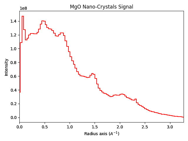
nano_crystals1d = nano_crystals.get_azimuthal_integral1d(npt=100, inplace=False)

nano_crystals1d.sum().plot()

"""
Similarly, the `get_azimuthal_integral2d` method will return a `Polar2D` signal.
"""

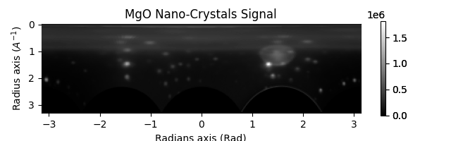
nano_crystals_polar = nano_crystals.get_azimuthal_integral2d(
    npt=100, npt_azim=360, inplace=False
)
nano_crystals_polar.sum().plot()

"""
There are also other things you can account for with azimuthal integration, such as the
effects of the Ewald sphere.  This can be done by calibrating with a known detector distance,
and beam energy.

Here we just show the effect of just calibrating with the first peak vs. calibrating
with the known beam energy and detector distance. For things like accurate template matching good
calibration can be important when matching to high diffraction vectors. The calibration example gives
more information on how to get the correct values for your microscope/setup.

If you are doing x-ray diffraction please raise an issue on the pyxem github to let us know! The same
assumptions should apply for each case, but it would be good to test!

We only show the 1D case here, but the same applies for the 2D case as well!
"""

nano_crystals.calibrate.detector(
    pixel_size=0.001,
    detector_distance=0.125,
    beam_energy=200,
    center=None,
    units="k_A^-1",
)  # set the center= None to use the center of the diffraction patterns
nano_crystals1d_200 = nano_crystals.get_azimuthal_integral1d(npt=100, inplace=False)
nano_crystals.calibrate.detector(
    pixel_size=0.001,
    detector_distance=0.075,
    beam_energy=80,
    center=None,
    units="k_A^-1",
)  # These are just made up pixel sizes and detector distances for illustration
nano_crystals1d_80 = nano_crystals.get_azimuthal_integral1d(npt=100, inplace=False)

hs.plot.plot_spectra(
    [nano_crystals1d.sum(), nano_crystals1d_200.sum(), nano_crystals1d_80.sum()],
    legend=["Flat Ewald Sphere Assumption", "200keV Corrected", "80keV Corrected"],
)

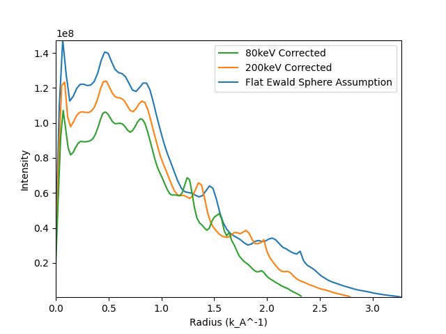
<Axes: xlabel='Radius (k_A^-1)', ylabel='Intensity'>

"""
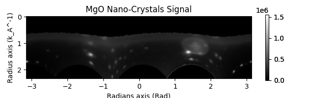
At times you may want to use a mask to exclude certain pixels from the azimuthal integration or apply an affine
transformation to the diffraction patterns before azimuthal integration.  This can be done using the `mask` and
`affine` parameters of the `Calibration` object.

Here we just show a random affine transformation for illustration.
"""

mask = nano_crystals.get_direct_beam_mask(radius=20)  # Mask the direct beam
affine = np.array(
    [[0.9, 0.1, 0], [0.1, 0.9, 0], [0, 0, 1]]
)  # Just a random affine transformation for illustration
nano_crystals.calibrate(mask=mask, affine=affine)
nano_crystals.get_azimuthal_integral2d(
    npt=100, npt_azim=360, inplace=False
).sum().plot()

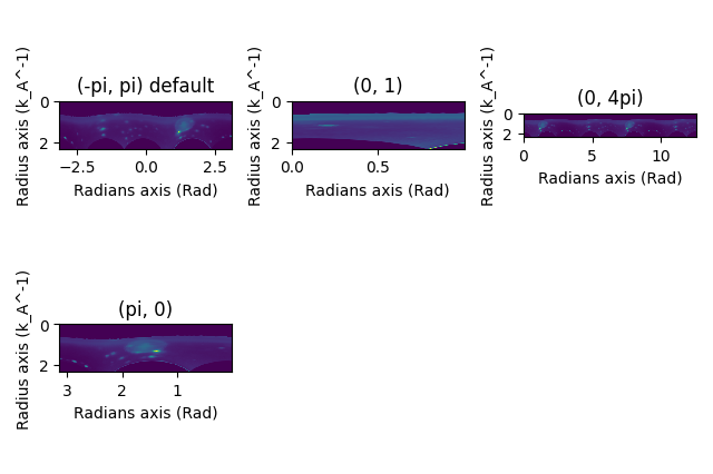
# The `azimuth_range`-argument lets you choose what angular range to calculate the azimuthal integral for.
# The range can be increasing, decreasing, and does not need to be a multiple of pi.

pol1 = nano_crystals.get_azimuthal_integral2d(npt=100, azimuth_range=(-np.pi, np.pi))

pol2 = nano_crystals.get_azimuthal_integral2d(npt=100, azimuth_range=(0, 1))

pol3 = nano_crystals.get_azimuthal_integral2d(
    npt=100, npt_azim=720, azimuth_range=(0, 4 * np.pi)
)

pol4 = nano_crystals.get_azimuthal_integral2d(npt=100, azimuth_range=(np.pi, 0))

hs.plot.plot_images(
    [pol1.sum(), pol2.sum(), pol3.sum(), pol4.sum()],
    label=["(-pi, pi) default", "(0, 1)", "(0, 4pi)", "(pi, 0)"],
    cmap="viridis",
    tight_layout=True,
    colorbar=None,
)

[<Axes: title={'center': '(-pi, pi) default'}, xlabel='Radians axis (Rad)', ylabel='Radius axis (k_A^-1)'>, <Axes: title={'center': '(0, 1)'}, xlabel='Radians axis (Rad)', ylabel='Radius axis (k_A^-1)'>, <Axes: title={'center': '(0, 4pi)'}, xlabel='Radians axis (Rad)', ylabel='Radius axis (k_A^-1)'>, <Axes: title={'center': '(pi, 0)'}, xlabel='Radians axis (Rad)', ylabel='Radius axis (k_A^-1)'>]