PDF Analysis Tutorial

Introduction

This tutorial demonstrates how to acquire a multidimensional pair distribution function (PDF) from both a flat field electron diffraction pattern and a scanning electron diffraction data set.

The data is from an open-source paper by Shanmugam et al. [1] that is used as a reference standard. It is an Amorphous 18nm SiO2 film. The scanning electron diffraction data set is a scan of a polycrystalline gold reference standard with 128x128 real space pixels and 256x256 diffraction space pixels. The implementation also initially followed Shanmugam et al.

[1] Shanmugam, J., Borisenko, K. B., Chou, Y. J., & Kirkland, A. I. (2017). eRDF Analyser: An interactive GUI for electron reduced density function analysis. SoftwareX, 6, 185-192.

This functionality has been checked to run in pyxem-0.15.0 (April 2023). Bugs are always possible, do not trust the code blindly, and if you experience any issues please report them here: pyxem/pyxem-demos#issues

Contents

1. Loading & Inspection

2. Acquiring a radial profile

3. Acquiring a Reduced Intensity

4. Damping the Reduced Intensity

5. Acquiring a PDF

Import pyXem and other required libraries

%matplotlib inline
import hyperspy.api as hs
import pyxem as pxm
import numpy as np

WARNING:silx.opencl.common:Unable to import pyOpenCl. Please install it from: https://pypi.org/project/pyopencl

1. Loading and Inspection

Load the diffraction data line profile

rp = hs.load('./data/08/amorphousSiO2.hspy')

WARNING:hyperspy.io:`signal_type='electron_diffraction1d'` not understood. See `hs.print_known_signal_types()` for a list of installed signal types or https://github.com/hyperspy/hyperspy-extensions-list for the list of all hyperspy extensions providing signals.
/Users/carterfrancis/mambaforge/envs/pyxem-demos/lib/python3.11/site-packages/hyperspy/misc/utils.py:471: VisibleDeprecationWarning: Use of the `binned` attribute in metadata is going to be deprecated in v2.0. Set the `axis.is_binned` attribute instead.
  warnings.warn(
/Users/carterfrancis/mambaforge/envs/pyxem-demos/lib/python3.11/site-packages/hyperspy/io.py:572: VisibleDeprecationWarning: Loading old file version. The binned attribute has been moved from metadata.Signal to axis.is_binned. Setting this attribute for all signal axes instead.
  warnings.warn('Loading old file version. The binned attribute '

rp.set_signal_type('electron_diffraction')

For now, the code requires navigation dimensions in the reduced intensity signal, two size 1 ones are created.

rp = pxm.signals.ElectronDiffraction1D([[rp.data]])

Set the diffraction pattern calibration. Note that pyXem uses a calibration to \(s = \frac{1}{d} = 2\frac{\sin{\theta}}{\lambda}\).

calibration = 0.00167

rp.set_diffraction_calibration(calibration=calibration)

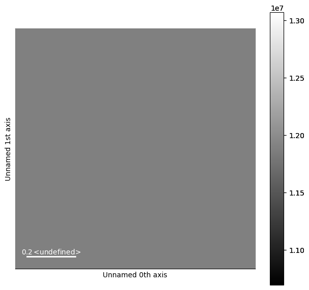
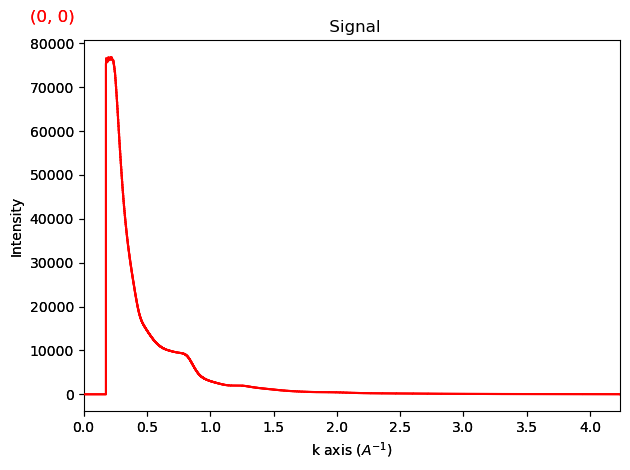
Plot the radial profile

rp.plot()

2. Acquiring a Reduced Intensity

Acquire a reduced intensity (also called a structure factor) from the radial profile. The structure factor is what will subsequently be transformed into a PDF through a fourier transform.

The structure factor \(\phi(s)\) is acquired by fitting a background scattering factor to the data, and then transforming the data by:

\[\phi(s) = \frac{I(s) - N\Delta c_{i}f_{i}^{2}}{N\Delta c_{i}^{2}f_{i}^{2}}\]

where s is the scattering vecot, \(c_{i}\) and \(f_{i}\) the atomic fraction and scattering factor respectively of each element in the sample, and N is a fitted parameter to the intensity.

To acquire the reduced intensity, we first initialise a ReducedIntensityGenerator1D object.

rigen = pxm.generators.ReducedIntensityGenerator1D(rp)

We then fit an electron scattering factor to the profile. To do this, we need to define a list of elements and their respective atomic fractions.

elements = ['Si','O']
fracs = [0.333,0.667]

Then we will fit a background scattering factor. The scattering factor parametrisation used here is that specified by Lobato and Van Dyck [2]. The plot_fit parameter ensures we check the fitted profile.

[2] Lobato, I., & Van Dyck, D. (2014). An accurate parameterization for scattering factors, electron densities and electrostatic potentials for neutral atoms that obey all physical constraints. Acta Crystallographica Section A: Foundations and Advances, 70(6), 636-649.

rigen.fit_atomic_scattering(elements,fracs,scattering_factor='lobato',plot_fit=True,iterpath='serpentine')

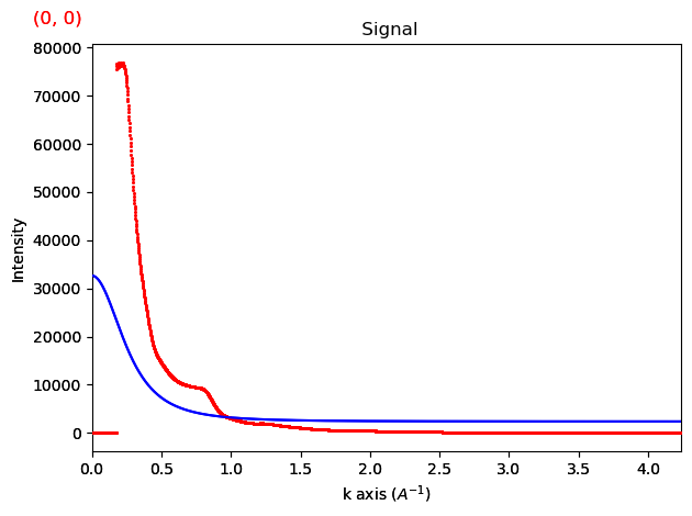
That’s clearly a terrible fit! This is because we’re trying to fit the beam stop. To avoid this, we specify to fit to the ‘tail end’ of the data by specifying a minimum and maximum scattering angle range. This is generally recommended, as electron scattering factors tend to not include inelastic scattering, which means the factors are rarely perfect fits.

rigen.set_s_cutoff(s_min=1.5,s_max=4)

rigen.fit_atomic_scattering(elements,fracs,scattering_factor='lobato',plot_fit=True,iterpath='serpentine')

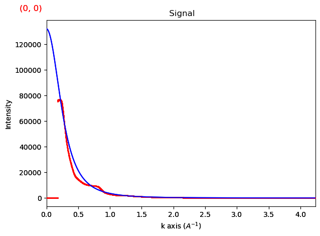
That’s clearly much much better. Always inspect your fit.

Finally, we calculate the reduced intensity itself.

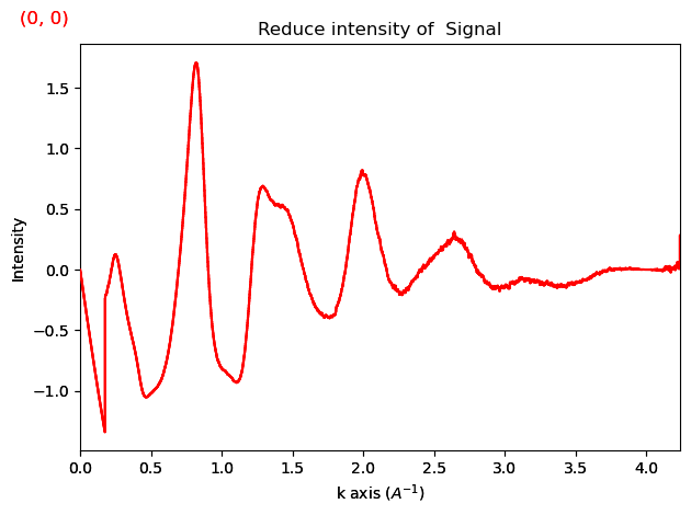
ri = rigen.get_reduced_intensity()

ri.plot()

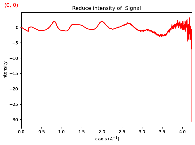
If it seems like the reduced intensity is not oscillating around 0 at high s, you should try fitting with a larger s_min. This generally speaking solves the issue.

4. Damping the Reduced Intensity

The reduced intensity acquired above does not go to zero at high s as it should because the maximum acquired scattering vector is not very high.

This would result in significant oscillation in the PDF due to a discontinuity in the fourier transformed data. To combat this, the reduced intensity is damped. In the X-ray community a common damping functions are the Lorch function and an exponential damping function. Both are supported here.

It is worth noting that damping does reduce the resolution in r in the PDF.

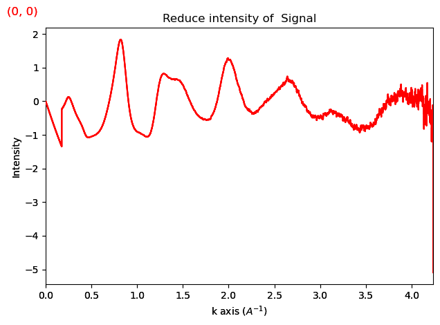
ri.damp_exponential(b=0.1)
ri.plot()

WARNING:hyperspy.io:`signal_type='reduced_intensity'` not understood. See `hs.print_known_signal_types()` for a list of installed signal types or https://github.com/hyperspy/hyperspy-extensions-list for the list of all hyperspy extensions providing signals.

[########################################] | 100% Completed | 105.80 ms

ri.damp_lorch(s_max=4)
ri.plot()

WARNING:hyperspy.io:`signal_type='reduced_intensity'` not understood. See `hs.print_known_signal_types()` for a list of installed signal types or https://github.com/hyperspy/hyperspy-extensions-list for the list of all hyperspy extensions providing signals.

[########################################] | 100% Completed | 106.11 ms

/Users/carterfrancis/mambaforge/envs/pyxem-demos/lib/python3.11/site-packages/pyxem/utils/ri_utils.py:118: RuntimeWarning: invalid value encountered in divide
  damping_term = np.sin(delta * scattering_axis) / (delta * scattering_axis)
/Users/carterfrancis/mambaforge/envs/pyxem-demos/lib/python3.11/site-packages/pyxem/utils/ri_utils.py:118: RuntimeWarning: invalid value encountered in divide
  damping_term = np.sin(delta * scattering_axis) / (delta * scattering_axis)

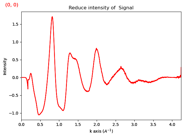
Additionally, it is recommended to damp the low s regime. We use an error function to do that

ri.damp_low_q_region_erfc(offset=4)
ri.plot()

WARNING:hyperspy.io:`signal_type='reduced_intensity'` not understood. See `hs.print_known_signal_types()` for a list of installed signal types or https://github.com/hyperspy/hyperspy-extensions-list for the list of all hyperspy extensions providing signals.

[########################################] | 100% Completed | 106.04 ms

If the function ends up overdamped, you can simply reacquire the reduced intensity using:

ri = rigen.get_reduced_intensity()

5. Acquiring a PDF

Finally, a PDF is acquired from the damped reduced intensity. This is done by a fourier sine transform. To ignore parts of the scattering data that are too noisy, you can set a minimum and maximum scattering angle for the transform.

First, we initialise a PDFGenerator1D object.

pdfgen = pxm.generators.PDFGenerator1D(ri)

/Users/carterfrancis/mambaforge/envs/pyxem-demos/lib/python3.11/site-packages/pyxem/generators/pdf_generator1d.py:39: VisibleDeprecationWarning: Function `__init__()` is deprecated and will be removed in version 1.0.0. Use `pyxem.signals.diffraction2d.get_pdf()` instead.
  since="0.15",

Secify a minimum and maximum scattering angle. The maximum must be equivalent to the Lorch function s_max if the Lorch function is used to damp. Otherwise the Lorch function damping can cause artifact in the PDF.

s_min = 0.
s_max = 4.

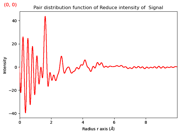
Finally we get the PDF. r_max specifies the maximum real space distance we want to interpret.

pdf = pdfgen.get_pdf(s_min=s_min, s_max=s_max, r_max=10)

/Users/carterfrancis/mambaforge/envs/pyxem-demos/lib/python3.11/site-packages/pyxem/generators/pdf_generator1d.py:47: VisibleDeprecationWarning: Function `get_pdf()` is deprecated and will be removed in version 1.0.0. Use `pyxem.signals.diffraction2d.get_pdf()` instead.
  since="0.15",

pdf.plot()

The PDF can then be saved.

pdf.save('Demo-PDF.hspy')