Data Inspection- Preprocessing - Unsupervised ML

This tutorial demonstrates the most important basic steps involved in the analysis of scanning electron diffraction data.

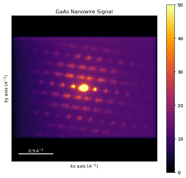
The data was acquired from a GaAs nanowire adopting the zinc blende structure and exhibiting type I twinning (i.e. on {111}) along its length. The region of interest contains a single nanowire comprising multiple crystals each in one of the two twinned orientations and near to a <1-10> zone axis.

This functionaility has been checked to run in pyxem version 0.14.1 (April 2022). However, bugs are always possible, do not trust the code blindly, and if you experience any issues please report them here: pyxem/pyxem-demos#issues

Contents

1. Loading & Inspection

2. Alignment & Calibration

3. Virtual Diffraction Imaging

4. Machine Learning SPED Data

5. Peak Finding

Import pyxem and other required libraries

# Changing the matplotlib background will give you interactive
#%matplotlib qt5

%matplotlib inline
import hyperspy.api as hs
import pyxem as pxm
import numpy as np

WARNING:silx.opencl.common:Unable to import pyOpenCl. Please install it from: https://pypi.org/project/pyopencl

1. Loading and Inspection

Load the SPED data acquired from the nanowire

dp = hs.load('./data/01/twinned_nanowire.hdf5', reader="hspy")

/Users/carterfrancis/mambaforge/envs/pyxem-demos/lib/python3.11/site-packages/hyperspy/misc/utils.py:471: VisibleDeprecationWarning: Use of the `binned` attribute in metadata is going to be deprecated in v2.0. Set the `axis.is_binned` attribute instead.
  warnings.warn(
/Users/carterfrancis/mambaforge/envs/pyxem-demos/lib/python3.11/site-packages/hyperspy/io.py:572: VisibleDeprecationWarning: Loading old file version. The binned attribute has been moved from metadata.Signal to axis.is_binned. Setting this attribute for all signal axes instead.
  warnings.warn('Loading old file version. The binned attribute '

Inspect the dp object

dp

<Diffraction2D, title: , dimensions: (30, 100|144, 144)>

Specify that the data is electron diffraction data

dp.set_signal_type('electron_diffraction')

Inspect the signal type

dp

<ElectronDiffraction2D, title: , dimensions: (30, 100|144, 144)>

Inspect the data type of the object

dp.data.dtype

dtype('uint8')

Inspect the metadata associated with the object ‘dp’

dp.metadata

Acquisition_instrument
TEM
• beam_energy = 300.0
• camera_length = 0.21000000000000002
• scan_rotation = 277.0

General
FileIO
0
• hyperspy_version = 1.7.5
• io_plugin = hyperspy.io_plugins.hspy
• operation = load
• timestamp = 2023-10-26T10:27:31.436805-05:00
• original_filename = nanowire_precession.blo
• time = (2014, 12, 8)
• title =

Signal
• signal_origin =
• signal_type = electron_diffraction

Set important experimental parameters using the built in function

dp.set_experimental_parameters(beam_energy=300.0,
                               camera_length=21.0,
                               scan_rotation=277.0,
                               convergence_angle=0.7,
                               exposure_time=10.0)

See how this changed the metadata

dp.metadata

Acquisition_instrument
TEM
Detector
Diffraction
• camera_length = 21.0
• exposure_time = 10.0
• beam_energy = 300.0
• camera_length = 0.21000000000000002
• convergence_angle = 0.7
• scan_rotation = 277.0

General
FileIO
0
• hyperspy_version = 1.7.5
• io_plugin = hyperspy.io_plugins.hspy
• operation = load
• timestamp = 2023-10-26T10:27:31.436805-05:00
• original_filename = nanowire_precession.blo
• time = (2014, 12, 8)
• title =

Signal
• signal_origin =
• signal_type = electron_diffraction

Set another metadata item and check it

dp.metadata.set_item("General.title", 'GaAs Nanowire')
dp.metadata

Acquisition_instrument
TEM
Detector
Diffraction
• camera_length = 21.0
• exposure_time = 10.0
• beam_energy = 300.0
• camera_length = 0.21000000000000002
• convergence_angle = 0.7
• scan_rotation = 277.0

General
FileIO
0
• hyperspy_version = 1.7.5
• io_plugin = hyperspy.io_plugins.hspy
• operation = load
• timestamp = 2023-10-26T10:27:31.436805-05:00
• original_filename = nanowire_precession.blo
• time = (2014, 12, 8)
• title = GaAs Nanowire

Signal
• signal_origin =
• signal_type = electron_diffraction

dp

<ElectronDiffraction2D, title: GaAs Nanowire, dimensions: (30, 100|144, 144)>

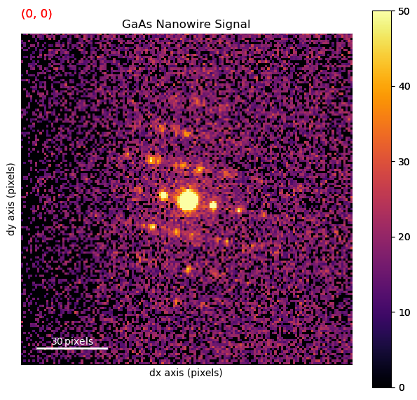
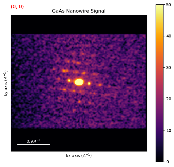
Plot the data to inspect it

dp.plot(cmap='inferno', vmax=50)

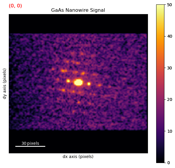
2. Alignment & Calibration

Apply distortion corrections to the data due to off-axis acquisition

dp.apply_affine_transformation(np.array([[0.99,0,0],
                                         [0,0.69,0],
                                         [0,0,1]]),
                               keep_dtype=True)

[########################################] | 100% Completed | 2.50 ss

dp.data.dtype

dtype('uint8')

Align the dataset based on the direct beam position

dp.center_direct_beam(method='cross_correlate',
                      radius_start=2,
                      radius_finish=5,
                      half_square_width=10)

[########################################] | 100% Completed | 32.64 s
[########################################] | 100% Completed | 1.99 ss

dp.plot(cmap='inferno', vmax=50)

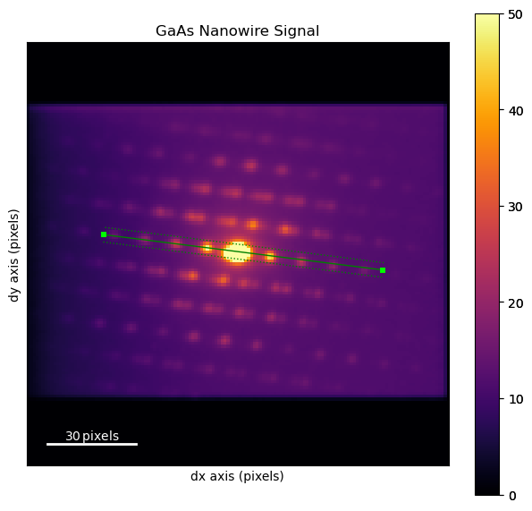
Measure known interplanar spacing to obtain calibration

dpm = dp.mean((0,1))
dpm.plot(cmap='inferno', vmax=50)
line = hs.roi.Line2DROI(x1=25.8525, y1=64.5691, x2=120.907, y2=77.0079, linewidth=5.49734)
line.add_widget(dpm)

<hyperspy.drawing._widgets.line2d.Line2DWidget at 0x1574b0290>

trace = line(dpm)
trace.plot()

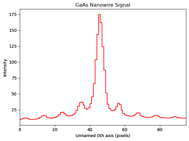
recip_d111 = np.sqrt((3/5.6535**2))
recip_cal = recip_d111 / 11.4

Set data calibrations

dp.set_diffraction_calibration(recip_cal)
dp.set_scan_calibration(10)

Plot the calibrated data

dp.plot(cmap='inferno', vmax=50)

3. Virtual Diffraction Imaging & Selecting Regions

3.1 Interactive VDF Imaging

Plot an interactive virtual image integrating intensity within a circular subset of pixels in the diffraction pattern

roi = hs.roi.CircleROI(cx=0.,cy=0, r_inner=0, r=0.07)

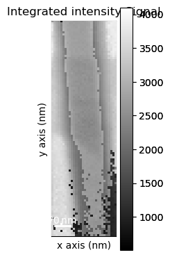
dp.plot_integrated_intensity(roi)

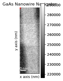
Get the virtual diffraction image associated with the last integration window used interactively

vdf = dp.get_integrated_intensity(roi)

Plot the virtual dark-field image

vdf.plot()

Inspect the metadata

vdf.metadata

Acquisition_instrument
TEM
Detector
Diffraction
• camera_length = 21.0
• exposure_time = 10.0
• beam_energy = 300.0
• camera_length = 0.21000000000000002
• convergence_angle = 0.7
• scan_rotation = 277.0

Diffraction
• integrated_range = CircleROI(cx=0, cy=0, r=0.07, r_inner=0) of GaAs Nanowire

General
FileIO
0
• hyperspy_version = 1.7.5
• io_plugin = hyperspy.io_plugins.hspy
• operation = load
• timestamp = 2023-10-26T10:27:31.436805-05:00
• original_filename = nanowire_precession.blo
• time = (2014, 12, 8)
• title = Integrated intensity

Signal
• signal_origin =
• signal_type =

Save the virtual dark-field image as a 32bit tif

vdf.change_dtype('float32')
vdf.save('vdfeg.tif')

3.2 Form multiple images using a VDF Generator

Import the VirtualImageGenerator class

from pyxem.generators.virtual_image_generator import VirtualImageGenerator

Initialize the VDFGenerator

vdfgen = VirtualImageGenerator(dp)

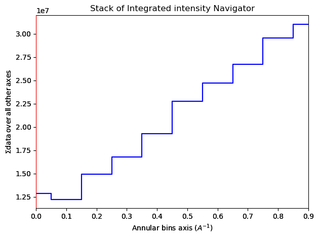
Calculate 10 annular VDF images between 0 and 1 reciprocal angstroms

vdfs = vdfgen.get_concentric_virtual_images(k_min=0,
                                        k_max=1,
                                        k_steps=10)

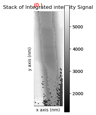
Plot the VDF images

vdfs.plot()

Save the stack of VDF image as a 32bit tif stack

vdfs.change_dtype('float32')
vdfs.save('vdsfeg.tif')

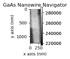
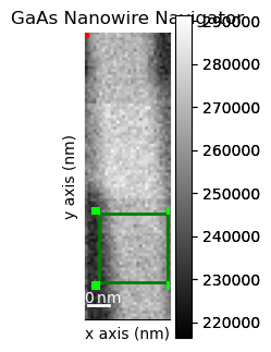
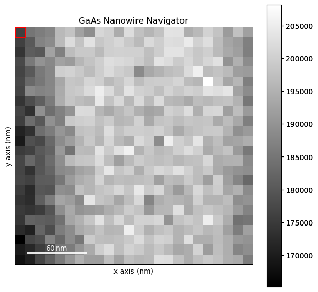
3.3 Select a region in the scan

Plot the data with an adjustable marker indicating where to crop the scan region

reg = hs.roi.RectangularROI(left=50, top=630, right=290, bottom=870)
dp.plot(cmap='inferno', vmax=50)
reg.add_widget(dp)

<hyperspy.drawing._widgets.rectangles.RectangleWidget at 0x157384150>

Crop the dataset based on the region defined above

dpc = reg(dp)

Calculate the mean diffraction pattern from the selected region

dpcm = dpc.mean((0,1))

Plot the mean diffraction pattern from the selected region

dpcm.plot(cmap='inferno', vmax=50)

4. Unsupervised learning

Perform singular value decomposition (SVD) of the data

dpc.data =dpc.data+1 # Sometimes the SVD Solver won't converge if there are a lot of zeros.

dpc.data = dpc.data.astype('float64')
dpc.decomposition(True, algorithm='SVD')

Decomposition info:
  normalize_poissonian_noise=True
  algorithm=SVD
  output_dimension=None
  centre=None

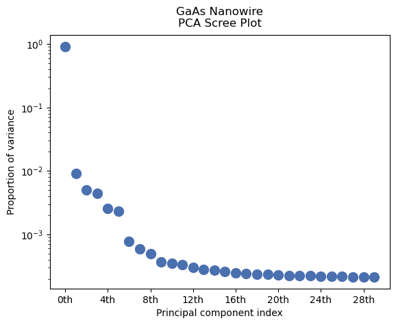
Obtain a “Scree plot” by plotting the fraction of variance described by each principal component

dpc.plot_explained_variance_ratio()

<Axes: title={'center': 'GaAs Nanowire\nPCA Scree Plot'}, xlabel='Principal component index', ylabel='Proportion of variance'>

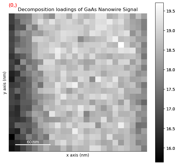
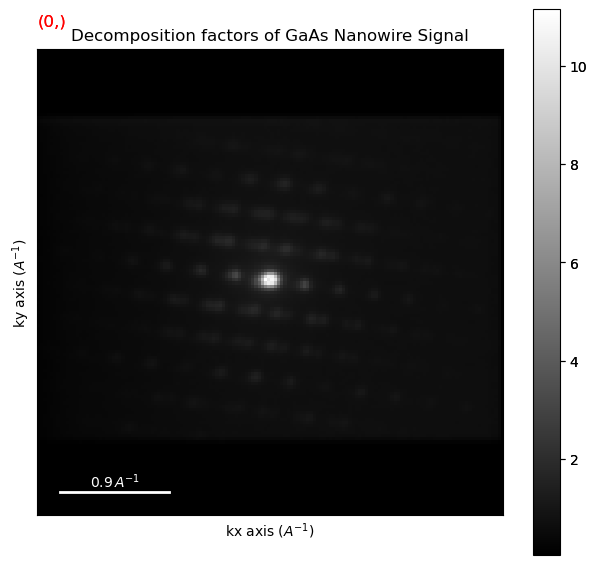
Plot the decomposition results and have a look at them

dpc.plot_decomposition_results()

WARNING:hyperspy.drawing.mpl_he:Navigation sliders not available. No toolkit registered. Install hyperspy_gui_ipywidgets or hyperspy_gui_traitsui GUI elements.

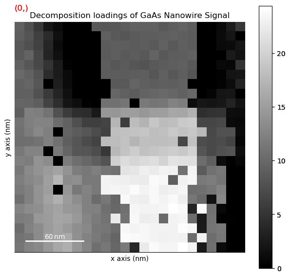
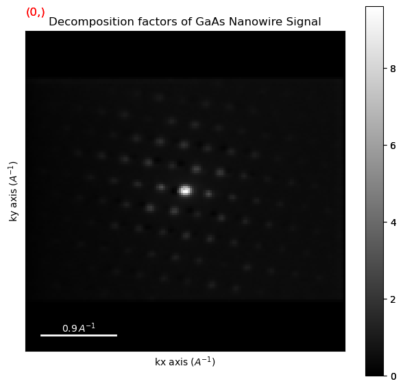
Perform non-negative matrix factorisation (NMF)

dpc.decomposition(True, algorithm='NMF', output_dimension=4,)

Decomposition info:
  normalize_poissonian_noise=True
  algorithm=NMF
  output_dimension=4
  centre=None
scikit-learn estimator:
NMF(n_components=4)

/Users/carterfrancis/mambaforge/envs/pyxem-demos/lib/python3.11/site-packages/sklearn/decomposition/_nmf.py:1710: ConvergenceWarning: Maximum number of iterations 200 reached. Increase it to improve convergence.
  warnings.warn(

Plot the NMF results

dpc.plot_decomposition_results()

WARNING:hyperspy.drawing.mpl_he:Navigation sliders not available. No toolkit registered. Install hyperspy_gui_ipywidgets or hyperspy_gui_traitsui GUI elements.

5. Peak Finding

Perform peak finding on all diffraction patterns in data

peaks = dpc.find_peaks(method='difference_of_gaussian',
                       min_sigma=1.,
                       max_sigma=6.,
                       sigma_ratio=1.6,
                       threshold=0.04,
                       overlap=0.99,
                       interactive=False)

[########################################] | 100% Completed | 3.47 ss

Check the peaks object type

peaks

<BaseSignal, title: GaAs Nanowire, dimensions: (24, 24|ragged)>

Look at what’s in the peaks object

print(peaks.inav[0,0].data)
print(" ")
print(peaks.inav[1,1].data)

[array([[60, 58],
        [70, 61],
        [61, 69],
        [71, 72],
        [82, 73],
        [73, 82],
        [83, 84]])]

[array([[59, 58],
        [70, 61],
        [61, 69],
        [71, 71],
        [82, 73],
        [73, 82],
        [83, 84]])]

coaxing peaks back into a DiffractionVectors

from pyxem.signals.diffraction_vectors import DiffractionVectors

peaks = DiffractionVectors.from_peaks(peaks,center=(72,72),calibration=recip_cal)

WARNING:hyperspy.signal:The function you applied does not take into account the difference of units and of scales in-between axes.

[########################################] | 100% Completed | 105.83 ms

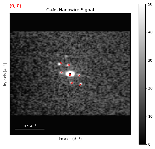
Plot found peak positions as an overlay on the data

peaks.plot_diffraction_vectors_on_signal(dpc, cmap='gray', vmax=50)

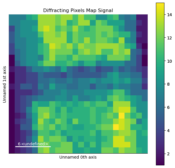
Form a diffracting pixels map to show where peaks were found and plot it

crystim = peaks.get_diffracting_pixels_map(binary=False)
crystim.plot(cmap='viridis')

WARNING:hyperspy.signal:The function you applied does not take into account the difference of units and of scales in-between axes.
WARNING:hyperspy.io:`signal_type='diffraction_vectors'` not understood. See `hs.print_known_signal_types()` for a list of installed signal types or https://github.com/hyperspy/hyperspy-extensions-list for the list of all hyperspy extensions providing signals.

[########################################] | 100% Completed | 106.79 ms

WARNING:hyperspy.io:`signal_type='signal2d'` not understood. See `hs.print_known_signal_types()` for a list of installed signal types or https://github.com/hyperspy/hyperspy-extensions-list for the list of all hyperspy extensions providing signals.