Phase/Orientation Mapping#
This tutorial demonstrates how to achieve phase and orientation mapping via scanning electron diffraction using both pattern and vector matching.
The data was acquired from a GaAs nanowire displaying polymorphism between zinc blende and wurtzite structures.
This functionaility has been checked to run in pyxem-0.13.0 (Feb 2021). Bugs are always possible, do not trust the code blindly, and if you experience any issues please report them here: pyxem/pyxem-demos#issues
Load & Inspect Data
Pre-processing
Template matching
[Build Template Library]
[Indexing]
Vector Matching
[Build Vector Library]
[Indexing Vectors]
Import pyxem and other required libraries
[ ]:
%matplotlib inline

import numpy as np
import diffpy.structure
import pyxem as pxm
import hyperspy.api as hs

accelarating_voltage = 200  # kV
camera_length = 0.2  # m
diffraction_calibration = 0.032  # px / Angstrom
WARNING:silx.opencl.common:Unable to import pyOpenCl. Please install it from: https://pypi.org/project/pyopencl
1. Loading and Inspection#
Load the demo data
[ ]:
dp = hs.load('./data/02/polymorphic_nanowire.hdf5', lazy=True)
dp
/Users/carterfrancis/mambaforge/envs/pyxem-dev/lib/python3.11/site-packages/hyperspy/misc/utils.py:471: VisibleDeprecationWarning: Use of the `binned` attribute in metadata is going to be deprecated in v2.0. Set the `axis.is_binned` attribute instead.
  warnings.warn(
/Users/carterfrancis/mambaforge/envs/pyxem-dev/lib/python3.11/site-packages/hyperspy/io.py:572: VisibleDeprecationWarning: Loading old file version. The binned attribute has been moved from metadata.Signal to axis.is_binned. Setting this attribute for all signal axes instead.
  warnings.warn('Loading old file version. The binned attribute '
|
|
Set data type, scale intensity range and set calibration
[ ]:
dp.data = dp.data.astype('float64')
dp.data *= 1 / dp.data.max()
Inspect metadata
[ ]:
dp.metadata
- Acquisition_instrument
- TEM
- Detector
- Diffraction
- camera_length = 10.0
- exposure_time = 10.0
- rocking_angle = 12.217304763960307
- rocking_frequency = 100.0
- scan_rotation = 1.0
- General
- FileIO
- 0
- hyperspy_version = 1.7.5
- io_plugin = hyperspy.io_plugins.hspy
- operation = load
- timestamp = 2023-11-06T13:07:24.894429-06:00
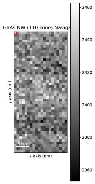
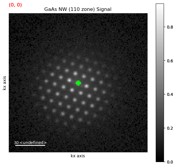
- title = GaAs NW (110 zone)
- Signal
- signal_type = electron_diffraction
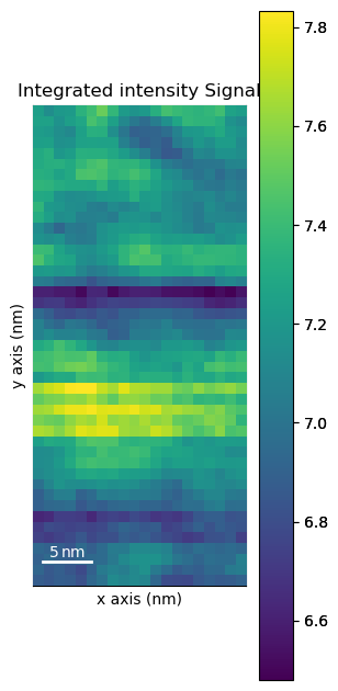
Plot an interactive virtual image to inspect data
[ ]:
roi = hs.roi.CircleROI(cx=72, cy=72, r_inner=0, r=2)
dp.plot_integrated_intensity(roi=roi, cmap='viridis')
[########################################] | 100% Completed | 317.33 ms
2. Pre-processing#
Apply affine transformation to correct for off axis camera geometry
[ ]:
scale_x = 0.995
scale_y = 1.031
offset_x = 0.631
offset_y = -0.351
dp.apply_affine_transformation(np.array([[scale_x, 0, offset_x],
                                         [0, scale_y, offset_y],
                                         [0, 0, 1]]))
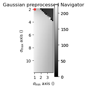
Perform difference of gaussian background subtraction with various parameters on one selected diffraction pattern and plot to identify good parameters
[ ]:
from pyxem.utils.expt_utils import investigate_dog_background_removal_interactive
[ ]:
dp_test_area = dp.inav[0, 0]

gauss_stddev_maxs = np.arange(2, 12, 0.2) # min, max, step
gauss_stddev_mins = np.arange(1, 4, 0.2) # min, max, step

investigate_dog_background_removal_interactive(dp_test_area,
                                               gauss_stddev_maxs,
                                               gauss_stddev_mins)
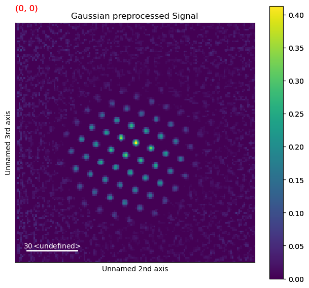
Remove background using difference of gaussians method with parameters identified above
[ ]:
dp = dp.subtract_diffraction_background('difference of gaussians',
                          min_sigma=2, max_sigma=8,
                          lazy_result=False)
[ ] | 0% Completed | 204.29 us
/Users/carterfrancis/mambaforge/envs/pyxem-dev/lib/python3.11/site-packages/pyxem/signals/diffraction2d.py:392: VisibleDeprecationWarning: Argument `lazy_result` is deprecated and will be removed in version 1.0.0. To avoid this warning, please do not use `lazy_result`. Use `lazy_output` instead. See the documentation of `subtract_diffraction_background()` for more details.
  name="lazy_result", alternative="lazy_output", since="0.15.0", removal="1.0.0"
[########################################] | 100% Completed | 954.47 ms
Perform further adjustments to the data ranges
[ ]:
dp.data -= dp.data.min()
dp.data *= 1 / dp.data.max()
Set diffraction calibration and scan calibration
[ ]:
dp = pxm.signals.ElectronDiffraction2D(dp) #this is needed because of a bug in the code
dp.set_diffraction_calibration(diffraction_calibration)
dp.set_scan_calibration(10)
3. Pattern Matching#
Pattern matching generates a database of simulated diffraction patterns and then compares all simulated patterns against each experimental pattern to find the best match
Import generators required for simulation and indexation
[ ]:
from diffsims.libraries.structure_library import StructureLibrary
from diffsims.generators.diffraction_generator import DiffractionGenerator
from diffsims.generators.library_generator import DiffractionLibraryGenerator

from diffsims.generators.zap_map_generator import get_rotation_from_z_to_direction
from diffsims.generators.rotation_list_generators import get_grid_around_beam_direction

from pyxem.generators.indexation_generator import AcceleratedIndexationGenerator
from pyxem.utils.indexation_utils import results_dict_to_crystal_map
3.1. Define Library of Structures & Orientations#
Define the crystal phases to be included in the simulated library
[ ]:
structure_zb = diffpy.structure.loadStructure('./data/02/GaAs_mp-2534_conventional_standard.cif')
structure_wz = diffpy.structure.loadStructure('./data/02/GaAs_mp-8883_conventional_standard.cif')
Create a basic rotations list.
Construct a StructureLibrary defining crystal structures and orientations for which diffraction will be simulated
[ ]:
[ ]:
struc_lib = StructureLibrary(['ZB','WZ'],
                             [structure_zb,structure_wz],
                             [rot_list_cubic,rot_list_hex])
### 3.2. Simulate Diffraction for all Structures & Orientations
Define a diffsims DiffractionGenerator with diffraction simulation parameters
[ ]:
diff_gen = DiffractionGenerator(accelerating_voltage=accelarating_voltage)
Initialize a diffsims DiffractionLibraryGenerator
Calulate library of diffraction patterns for all phases and unique orientations
[ ]:
target_pattern_dimension_pixels = dp.axes_manager.signal_shape[0]
half_size = target_pattern_dimension_pixels // 2
reciprocal_radius = diffraction_calibration*(half_size - 1)

diff_lib = lib_gen.get_diffraction_library(struc_lib,
                                           calibration=diffraction_calibration,
                                           reciprocal_radius=reciprocal_radius,
                                           half_shape=(half_size, half_size),
                                           max_excitation_error=1/10,
                                           with_direct_beam=False)
Optionally, save the library for later use.
[ ]:
diff_lib.pickle_library('./GaAs_cubic_hex.pickle')
If saved, the library can be loaded as follows
[ ]:
from diffsims.libraries.diffraction_library import load_DiffractionLibrary
diff_lib = load_DiffractionLibrary('./GaAs_cubic_hex.pickle', safety=True)
### 3.3. Pattern Matching Indexation
Initialize TemplateIndexationGenerator with the experimental data and diffraction library and perform correlation, returning the n_largest matches with highest correlation.
Note: Try using the workflow from 11 Accelerated Orientation Mapping
[ ]:
indexer = AcceleratedIndexationGenerator(dp, diff_lib)
indexation_results,phase_dict  = indexer.correlate(n_largest=3)
[ ] | 0% Completed | 1.68 s ms
OMP: Info #276: omp_set_nested routine deprecated, please use omp_set_max_active_levels instead.
[########################################] | 100% Completed | 3.98 s
Check the solutions via a plotting (can be slow, so we don’t run by default)
[ ]:
#if False:
#    indexation_results.plot_best_matching_results_on_signal(dp, diff_lib)
Get crystallographic map from indexation results
[ ]:
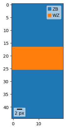
crystal_map = results_dict_to_crystal_map(indexation_results, phase_key_dict=phase_dict)
crystal_map is now a CrystalMap object, which comes from orix, see their documentation for details. Below we lift their code to plot a phase map
[ ]:
from matplotlib import pyplot as plt
from orix import plot

fig, ax = plt.subplots(subplot_kw=dict(projection="plot_map"))
im = ax.plot_map(crystal_map)
4. Vector Matching#
Note: This workflow is less well developed than the template matching one, and may well be broken
Vector matching generates a database of vector pairs (magnitues and inter-vector angles) and then compares all theoretical values against each measured diffraction vector pair to find the best match
Import generators required for simulation and indexation
[ ]:
#from diffsims.generators.library_generator import VectorLibraryGenerator
#from diffsims.libraries.structure_library import StructureLibrary
#from diffsims.libraries.vector_library import load_VectorLibrary

#from pyxem.generators.indexation_generator import VectorIndexationGenerator

#from pyxem.generators.subpixelrefinement_generator import SubpixelrefinementGenerator
#from pyxem.signals.diffraction_vectors import DiffractionVectors
### 4.1. Define Library of Structures
Define crystal structure for which to determine theoretical vector pairs
[ ]:
#structure_zb = diffpy.structure.loadStructure('./data/02/GaAs_mp-2534_conventional_standard.cif')
#structure_wz = diffpy.structure.loadStructure('./data/02/GaAs_mp-8883_conventional_standard.cif')

#structure_library = StructureLibrary(['ZB', 'WZ'],
#                                     [structure_zb, structure_wz],
#                                     [[], []])
Initialize VectorLibraryGenerator with structures to be considered
[ ]:
#vlib_gen = VectorLibraryGenerator(structure_library)
Determine VectorLibrary with all vectors within given reciprocal radius
[ ]:
#reciprocal_radius = diffraction_calibration*(half_size - 1)

#vec_lib = vlib_gen.get_vector_library(reciprocal_radius)
Optionally, save the library for later use
[ ]:
#vec_lib.pickle_library('./GaAs_cubic_hex_vectors.pickle')
[ ]:
#vec_lib = load_VectorLibrary('./GaAs_cubic_hex_vectors.pickle',safety=True)
4.2. Find Diffraction Peaks#
Tune peak finding parameters interactively
[ ]:
#dp.find_peaks(interactive=False)
Perform peak finding on the data with parameters from above
[ ]:
#peaks = dp.find_peaks(method='difference_of_gaussian',
#                      min_sigma=0.005,
#                      max_sigma=5.0,
#                      sigma_ratio=2.0,
#                      threshold=0.06,
#                      overlap=0.8,
#                      interactive=False)
coaxing peaks back into a DiffractionVectors
[ ]:
#peaks = DiffractionVectors(peaks).T
peaks now contain the 2D positions of the diffraction spots on the detector. The vector matching method works in 3D coordinates, which are found by projecting the detector positions back onto the Ewald sphere. Because the methods that follow are slow, we constrain ourselves to looking at a smaller subset of the data
[ ]:
#peaks = peaks.inav[:2,:2]
[ ]:
#peaks.calculate_cartesian_coordinates?
[ ]:
#peaks.calculate_cartesian_coordinates(accelerating_voltage=accelarating_voltage,
#                                      camera_length=camera_length)
### 4.3. Vector Matching Indexation
Initialize VectorIndexationGenerator with the experimental data and vector library and perform indexation using n_peaks_to_index and returning the n_best indexation results.
Alert: This code no longer works on this example, and may even be completely broken. Caution is advised.
[ ]:
#indexation_generator = VectorIndexationGenerator(peaks, vec_lib)
[ ]:
#indexation_results = indexation_generator.index_vectors(mag_tol=3*diffraction_calibration,
#                                                        angle_tol=4,  # degree
#                                                        index_error_tol=0.2,
#                                                        n_peaks_to_index=7,
#                                                        n_best=5,
#                                                        show_progressbar=True)
[ ]:
#indexation_results.data
Refine all crystal orientations for improved phase reliability and orientation reliability maps.
[ ]:
#refined_results = indexation_generator.refine_n_best_orientations(indexation_results,
#                                                                  accelarating_voltage=accelarating_voltage,
#                                                                  camera_length=camera_length,
#                                                                  index_error_tol=0.2,
#                                                                  vary_angles=True,
#                                                                  vary_scale=True,
#                                                                  method="leastsq")"""
Get crystallographic map from optimized indexation results.
[ ]:
#crystal_map = refined_results.get_crystallographic_map()
See the objections documentation for further details
[ ]:
#crystal_map?