Nanocrystal Segmentation#

This notebook demonstrates two approaches to nanocrystal segmentation: 1. Virtual dark-field (VDF) imaging-based segmentation 2. Non-negative matrix factorisation (NMF)-based segmentation

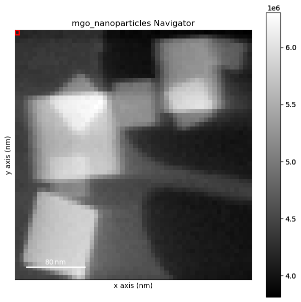
The segmentation is demonstrated on a SPED dataset of partly overlapping MgO nanoparticles, where some of the particles share the same orientation.

This functionality has been checked to run with pyxem-0.15.0 (April 2023). Bugs are always possible, do not trust the code blindly, and if you experience any issues please report them here: pyxem/pyxem-demos#issues

Contents#

Setting up, Loading Data, Pre-processing
Virtual Image Based Segmentation
NMF Based Segmentation

1. Setting up, Loading Data, Pre-processing#

Import pyxem and other required libraries

[ ]:

%matplotlib inline
import numpy as np
import hyperspy.api as hs
import matplotlib.pyplot as plt
import pyxem as pxm

WARNING:silx.opencl.common:The module pyOpenCL has been imported but can't be used here

Load demonstration data

[ ]:

dp = hs.load('./data/06/mgo_nanoparticles.hdf5', reader="hspy")

/home/cssfrancis/hyperspy-bundle/lib/python3.10/site-packages/hyperspy/misc/utils.py:471: VisibleDeprecationWarning: Use of the `binned` attribute in metadata is going to be deprecated in v2.0. Set the `axis.is_binned` attribute instead.
  warnings.warn(
/home/cssfrancis/hyperspy-bundle/lib/python3.10/site-packages/hyperspy/io.py:572: VisibleDeprecationWarning: Loading old file version. The binned attribute has been moved from metadata.Signal to axis.is_binned. Setting this attribute for all signal axes instead.
  warnings.warn('Loading old file version. The binned attribute '

Set the Calibrations…

[ ]:

scale = 0.03246*2
scale_real = 3.03*2
dp.set_diffraction_calibration(scale)
dp.set_scan_calibration(scale_real)

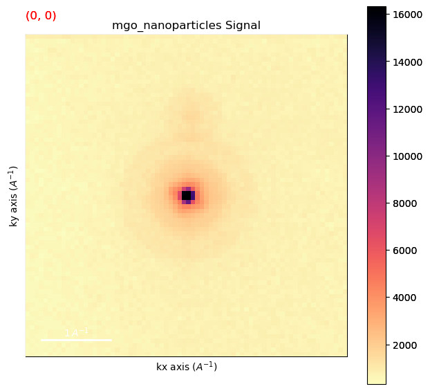
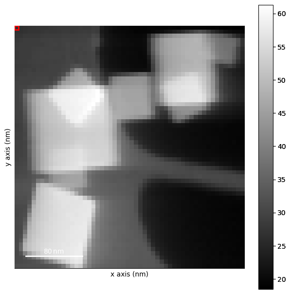
Plot data to inspect

[ ]:

%matplotlib inline
dp.plot(cmap='magma_r')

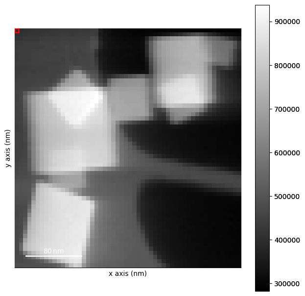
../../_images/tutorials_pyxem-demos_06_Nanocrystal_segmentation_in_SPED_data_-_Demonstration_on_partly_overlapping_MgO_cubes_14_0.png

../../_images/tutorials_pyxem-demos_06_Nanocrystal_segmentation_in_SPED_data_-_Demonstration_on_partly_overlapping_MgO_cubes_14_1.png

Remove the background

[ ]:

sigma_min = 1.7
sigma_max = 13.2

dp_rb= dp.subtract_diffraction_background('difference of gaussians',
                             min_sigma=sigma_min,
                             max_sigma=sigma_max)
dp_rb.set_signal_type("electron_diffraction") # This will be fixed with pyxem/pyxem#889

[########################################] | 100% Completed | 911.32 ms

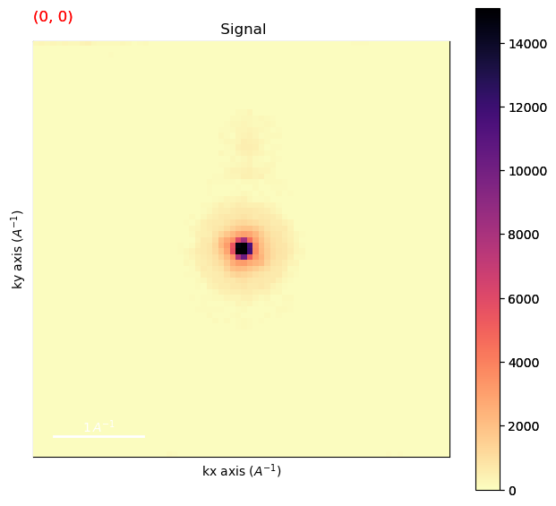
Plot the background subtracted data

[ ]:

dp_rb.plot(cmap='magma_r')

../../_images/tutorials_pyxem-demos_06_Nanocrystal_segmentation_in_SPED_data_-_Demonstration_on_partly_overlapping_MgO_cubes_18_0.png

../../_images/tutorials_pyxem-demos_06_Nanocrystal_segmentation_in_SPED_data_-_Demonstration_on_partly_overlapping_MgO_cubes_18_1.png

Find the position of the direct beam in the background subtracted data.

[ ]:

shifts  = dp_rb.get_direct_beam_position(method='blur',
                                         signal_slice=(-.4, .4,-.4,.4),
                                         sigma=2,)

[########################################] | 100% Completed | 505.80 ms

[ ]:

shifts

<BeamShift, title: , dimensions: (54, 57|2)>

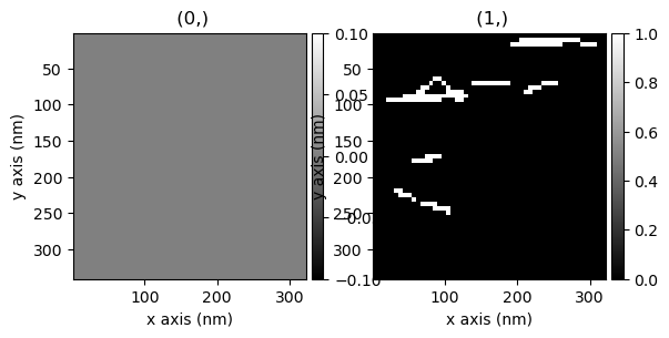
Visualizing the shifts. This gives us a better idea of what the shifts look like.

In this case the shifts are small (1 pixel or zero pixels in most cases)

[ ]:

hs.plot.plot_images(shifts.T)

[<Axes: title={'center': ' (0,)'}, xlabel='x axis (nm)', ylabel='y axis (nm)'>,
 <Axes: title={'center': ' (1,)'}, xlabel='x axis (nm)', ylabel='y axis (nm)'>]

../../_images/tutorials_pyxem-demos_06_Nanocrystal_segmentation_in_SPED_data_-_Demonstration_on_partly_overlapping_MgO_cubes_23_1.png

Apply the same shifts to the raw data.

[ ]:

dp_shifted = dp_rb.center_direct_beam(shifts=shifts, inplace=False)

[########################################] | 100% Completed | 303.59 ms

2. Virtual Image Based Segmentation#

2.1. Peak Finding & Refinement#

Find all diffraction peaks for all PED patterns. The parameters were found by interactive peak finding:

peaks = dp_rb.find_peaks_interactive(imshow_kwargs={'cmap': 'magma_r'})

[ ]:

import hyperspy
hyperspy.__version__

'1.7.5'

[ ]:

dp_shifted.data = dp_shifted.data/dp_shifted.max(axis=(0,1,2,3)).data

[ ]:

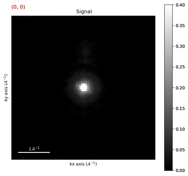
dp_shifted.plot(vmax=.4)

../../_images/tutorials_pyxem-demos_06_Nanocrystal_segmentation_in_SPED_data_-_Demonstration_on_partly_overlapping_MgO_cubes_32_0.png

../../_images/tutorials_pyxem-demos_06_Nanocrystal_segmentation_in_SPED_data_-_Demonstration_on_partly_overlapping_MgO_cubes_32_1.png

[ ]:

peaks = dp_shifted.find_peaks(method='minmax',
                         threshold=.03,
                         distance=3,

                         interactive=False)

[########################################] | 100% Completed | 2.34 ss

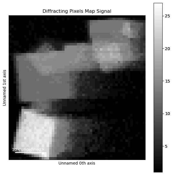
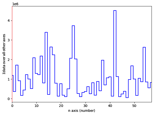
Visualise the number of diffraction peaks found at each probe position

[ ]:

from pyxem.signals.diffraction_vectors import DiffractionVectors
peaks = DiffractionVectors.from_peaks(peaks,center=(36,36),calibration=scale)

WARNING:hyperspy.signal:The function you applied does not take into account the difference of units and of scales in-between axes.

[########################################] | 100% Completed | 101.74 ms

[ ]:

diff_map = peaks.get_diffracting_pixels_map()
diff_map.plot()

WARNING:hyperspy.signal:The function you applied does not take into account the difference of units and of scales in-between axes.
WARNING:hyperspy.io:`signal_type='diffraction_vectors'` not understood. See `hs.print_known_signal_types()` for a list of installed signal types or https://github.com/hyperspy/hyperspy-extensions-list for the list of all hyperspy extensions providing signals.

[########################################] | 100% Completed | 101.61 ms

WARNING:hyperspy.io:`signal_type='signal2d'` not understood. See `hs.print_known_signal_types()` for a list of installed signal types or https://github.com/hyperspy/hyperspy-extensions-list for the list of all hyperspy extensions providing signals.

../../_images/tutorials_pyxem-demos_06_Nanocrystal_segmentation_in_SPED_data_-_Demonstration_on_partly_overlapping_MgO_cubes_36_3.png

Exclude peaks too close to the detector edge for sub-pixel refinement.

[ ]:

peaks.flatten_diffraction_vectors(real_units=False)

<DiffractionVectors2D, title: , dimensions: (|4, 23409)>

[ ]:

peaks.detector_shape = dp.axes_manager.signal_shape

[ ]:

peaks.scales[0]*(peaks.detector_shape[0]/2) - peaks.scales[0]*2

2.20728

[ ]:

peaks_filtered = peaks.filter_detector_edge(exclude_width=5)

WARNING:hyperspy.signal:The function you applied does not take into account the difference of units and of scales in-between axes.
WARNING:hyperspy.io:`signal_type='diffraction_vectors'` not understood. See `hs.print_known_signal_types()` for a list of installed signal types or https://github.com/hyperspy/hyperspy-extensions-list for the list of all hyperspy extensions providing signals.

[########################################] | 100% Completed | 101.45 ms

Refine the peak positions using center of mass

[ ]:

from pyxem.generators.subpixelrefinement_generator import SubpixelrefinementGenerator
from pyxem.signals.diffraction_vectors import DiffractionVectors

refine_gen = SubpixelrefinementGenerator(dp_rb, peaks_filtered)

peaks_refined = DiffractionVectors(refine_gen.center_of_mass_method(square_size=4))

WARNING:hyperspy.signal:The function you applied does not take into account the difference of units and of scales in-between axes.
WARNING:hyperspy.io:`signal_type='diffraction_vectors'` not understood. See `hs.print_known_signal_types()` for a list of installed signal types or https://github.com/hyperspy/hyperspy-extensions-list for the list of all hyperspy extensions providing signals.

[########################################] | 100% Completed | 102.81 ms

WARNING:hyperspy.io:`signal_type='diffraction_vectors'` not understood. See `hs.print_known_signal_types()` for a list of installed signal types or https://github.com/hyperspy/hyperspy-extensions-list for the list of all hyperspy extensions providing signals.

[########################################] | 100% Completed | 1.09 sms

[ ]:

peaks_filtered.scales

[0.06492, 0.06492]

2.2. Determine Unique Peaks#

Determine the unique diffraction peaks by clustering

[ ]:

peaks_filtered.scales

[0.06492, 0.06492]

[ ]:

def replace_nan(data):
    new_data = data
    new_data[np.isnan(data)]=0
    return np.array(new_data)

[ ]:

peaks_refined = peaks_refined.map(replace_nan, inplace=False, ragged=True)

WARNING:hyperspy.signal:The function you applied does not take into account the difference of units and of scales in-between axes.
WARNING:hyperspy.io:`signal_type='diffraction_vectors'` not understood. See `hs.print_known_signal_types()` for a list of installed signal types or https://github.com/hyperspy/hyperspy-extensions-list for the list of all hyperspy extensions providing signals.

[########################################] | 100% Completed | 101.09 ms

[ ]:

peaks_refined.scales

[ ]:

peaks_refined.set_signal_type("diffraction_vectors")

[ ]:

distance_threshold = scale*0.89*2
min_samples = 10

unique_peaks = peaks_refined.get_unique_vectors(method='DBSCAN',
                                                distance_threshold=distance_threshold,
                                                min_samples=min_samples)
print(np.shape(unique_peaks.data)[0], ' unique vectors were found.')

39  unique vectors were found.

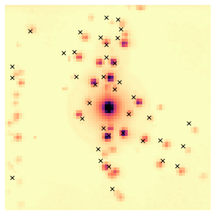
Visualise the detected unique peaks by plotting them on the maximum of the signal.

[ ]:

radius_px = dp_rb.axes_manager.signal_shape[0]/2
reciprocal_radius = radius_px * scale

[ ]:

dp_rb.axes_manager.signal_extent

(-2.33712, 2.2722, -2.33712, 2.2722)

[ ]:

peaks_refined.plot_diffraction_vectors(
    method='DBSCAN',
    unique_vectors=unique_peaks,
    distance_threshold=distance_threshold,
    xlim=reciprocal_radius,
    ylim=reciprocal_radius,
    min_samples=min_samples,
    image_to_plot_on=dp_rb.max(),
    image_cmap='magma_r',
    plot_label_colors=False)

../../_images/tutorials_pyxem-demos_06_Nanocrystal_segmentation_in_SPED_data_-_Demonstration_on_partly_overlapping_MgO_cubes_56_0.png

../../_images/tutorials_pyxem-demos_06_Nanocrystal_segmentation_in_SPED_data_-_Demonstration_on_partly_overlapping_MgO_cubes_56_1.png

Visualise both the clusters and the unique peaks obtained after DBSCAN clustering.

NB The cluster colors are randomly generated, so run it again if it is hard to discern two close clusters.

Filter the unique vectors by magnitude in order to exclude the direct beam from the following analysis

[ ]:

Gs = unique_peaks.filter_magnitude(min_magnitude=10*scale,
                                   max_magnitude=np.inf)
print(np.shape(Gs)[0], ' unique vectors.')

29  unique vectors.

This gets us a set of basis vectors. We can then plot where these vectors exsist in the dataset.

[ ]:

filtered = peaks_refined.filter_basis(Gs.data, distance=0.1, inplace=False)

WARNING:hyperspy.signal:The function you applied does not take into account the difference of units and of scales in-between axes.
WARNING:hyperspy.io:`signal_type='diffraction_vectors'` not understood. See `hs.print_known_signal_types()` for a list of installed signal types or https://github.com/hyperspy/hyperspy-extensions-list for the list of all hyperspy extensions providing signals.

[########################################] | 100% Completed | 102.66 ms

Optionally save and load the unique peaks

[ ]:

Gs.save("peaks.hspy", overwrite=True)

[ ]:

hs.load("peaks.hspy")

<DiffractionVectors2D, title: , dimensions: (|2, 29)>

2.3. Virtual Imaging & Segmentation#

Calculate VDF images for all unique peaks

[ ]:

from pyxem.generators import VirtualDarkFieldGenerator

radius=scale*2

vdfgen = VirtualDarkFieldGenerator(dp_rb, Gs)
VDFs = vdfgen.get_virtual_dark_field_images(radius=radius)
print(VDFs.vectors)
#VDFs.compute()
print(VDFs.vectors)
VDFs.metadata

<DiffractionVectors2D, title: , dimensions: (|2, 29)>
<DiffractionVectors2D, title: , dimensions: (|2, 29)>

Diffraction

roi_list <list>

[0] = CircleROI(cx=-0.06492, cy=-2.07744, r=0.12984, r_inner=0)

[1] = CircleROI(cx=0.20277, cy=-2.03756, r=0.12984, r_inner=0)

[10] = CircleROI(cx=-0.06492, cy=-1.17147, r=0.12984, r_inner=0)

[11] = CircleROI(cx=-0.127401, cy=-0.730211, r=0.12984, r_inner=0)

[12] = CircleROI(cx=0.12984, cy=-1.03843, r=0.12984, r_inner=0)

[13] = CircleROI(cx=-2.20728, cy=-0.960816, r=0.12984, r_inner=0)

[14] = CircleROI(cx=-0.746933, cy=-0.736649, r=0.12984, r_inner=0)

[15] = CircleROI(cx=-2.20728, cy=-0.711716, r=0.12984, r_inner=0)

[16] = CircleROI(cx=0.239604, cy=-0.607185, r=0.12984, r_inner=0)

[17] = CircleROI(cx=0.908523, cy=0.195794, r=0.12984, r_inner=0)

[18] = CircleROI(cx=1.81776, cy=0.332947, r=0.12984, r_inner=0)

[19] = CircleROI(cx=0.764287, cy=0.731048, r=0.12984, r_inner=0)

[2] = CircleROI(cx=0.264317, cy=-1.81173, r=0.12984, r_inner=0)

[20] = CircleROI(cx=1.16856, cy=0.710855, r=0.12984, r_inner=0)

[21] = CircleROI(cx=1.68692, cy=0.843625, r=0.12984, r_inner=0)

[22] = CircleROI(cx=-0.244657, cy=0.912099, r=0.12984, r_inner=0)

[23] = CircleROI(cx=-0.19476, cy=1.18182, r=0.12984, r_inner=0)

[24] = CircleROI(cx=1.22185, cy=1.18356, r=0.12984, r_inner=0)

[25] = CircleROI(cx=1.5477, cy=1.29881, r=0.12984, r_inner=0)

[26] = CircleROI(cx=-0.00808017, cy=1.30893, r=0.12984, r_inner=0)

[27] = CircleROI(cx=-2.20728, cy=1.56457, r=0.12984, r_inner=0)

[28] = CircleROI(cx=0.0704502, cy=1.81864, r=0.12984, r_inner=0)

[3] = CircleROI(cx=-1.79086, cy=-1.76881, r=0.12984, r_inner=0)

[4] = CircleROI(cx=-0.65321, cy=-1.75055, r=0.12984, r_inner=0)

[5] = CircleROI(cx=-0.195, cy=-1.62156, r=0.12984, r_inner=0)

[6] = CircleROI(cx=0.195144, cy=-1.61819, r=0.12984, r_inner=0)

[7] = CircleROI(cx=-0.06492, cy=-1.4607, r=0.12984, r_inner=0)

[8] = CircleROI(cx=-1.03872, cy=-1.27243, r=0.12984, r_inner=0)

[9] = CircleROI(cx=-0.787033, cy=-1.29628, r=0.12984, r_inner=0)

General

FileIO

0

hyperspy_version = 1.7.5

io_plugin = hyperspy.io_plugins.hspy

operation = load

timestamp = 2023-06-08T19:24:02.403562-05:00

title = Stack of Integrated intensity

Signal

signal_type = virtual_dark_field

Vectors = <DiffractionVectors2D, title: , dimensions: (|2, 29)>

[ ]:

VDFs.metadata

Diffraction

roi_list <list>

[0] = CircleROI(cx=-0.06492, cy=-2.07744, r=0.12984, r_inner=0)

[1] = CircleROI(cx=0.20277, cy=-2.03756, r=0.12984, r_inner=0)

[10] = CircleROI(cx=-0.06492, cy=-1.17147, r=0.12984, r_inner=0)

[11] = CircleROI(cx=-0.127401, cy=-0.730211, r=0.12984, r_inner=0)

[12] = CircleROI(cx=0.12984, cy=-1.03843, r=0.12984, r_inner=0)

[13] = CircleROI(cx=-2.20728, cy=-0.960816, r=0.12984, r_inner=0)

[14] = CircleROI(cx=-0.746933, cy=-0.736649, r=0.12984, r_inner=0)

[15] = CircleROI(cx=-2.20728, cy=-0.711716, r=0.12984, r_inner=0)

[16] = CircleROI(cx=0.239604, cy=-0.607185, r=0.12984, r_inner=0)

[17] = CircleROI(cx=0.908523, cy=0.195794, r=0.12984, r_inner=0)

[18] = CircleROI(cx=1.81776, cy=0.332947, r=0.12984, r_inner=0)

[19] = CircleROI(cx=0.764287, cy=0.731048, r=0.12984, r_inner=0)

[2] = CircleROI(cx=0.264317, cy=-1.81173, r=0.12984, r_inner=0)

[20] = CircleROI(cx=1.16856, cy=0.710855, r=0.12984, r_inner=0)

[21] = CircleROI(cx=1.68692, cy=0.843625, r=0.12984, r_inner=0)

[22] = CircleROI(cx=-0.244657, cy=0.912099, r=0.12984, r_inner=0)

[23] = CircleROI(cx=-0.19476, cy=1.18182, r=0.12984, r_inner=0)

[24] = CircleROI(cx=1.22185, cy=1.18356, r=0.12984, r_inner=0)

[25] = CircleROI(cx=1.5477, cy=1.29881, r=0.12984, r_inner=0)

[26] = CircleROI(cx=-0.00808017, cy=1.30893, r=0.12984, r_inner=0)

[27] = CircleROI(cx=-2.20728, cy=1.56457, r=0.12984, r_inner=0)

[28] = CircleROI(cx=0.0704502, cy=1.81864, r=0.12984, r_inner=0)

[3] = CircleROI(cx=-1.79086, cy=-1.76881, r=0.12984, r_inner=0)

[4] = CircleROI(cx=-0.65321, cy=-1.75055, r=0.12984, r_inner=0)

[5] = CircleROI(cx=-0.195, cy=-1.62156, r=0.12984, r_inner=0)

[6] = CircleROI(cx=0.195144, cy=-1.61819, r=0.12984, r_inner=0)

[7] = CircleROI(cx=-0.06492, cy=-1.4607, r=0.12984, r_inner=0)

[8] = CircleROI(cx=-1.03872, cy=-1.27243, r=0.12984, r_inner=0)

[9] = CircleROI(cx=-0.787033, cy=-1.29628, r=0.12984, r_inner=0)

General

FileIO

0

hyperspy_version = 1.7.5

io_plugin = hyperspy.io_plugins.hspy

operation = load

timestamp = 2023-06-08T19:24:02.403562-05:00

title = Stack of Integrated intensity

Signal

signal_type = virtual_dark_field

Vectors = <DiffractionVectors2D, title: , dimensions: (|2, 29)>

[ ]:

VDFs.set_signal_type("virtual_dark_field")

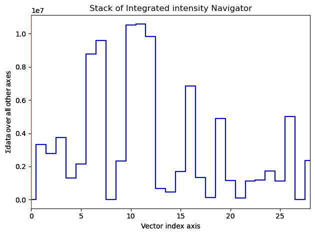
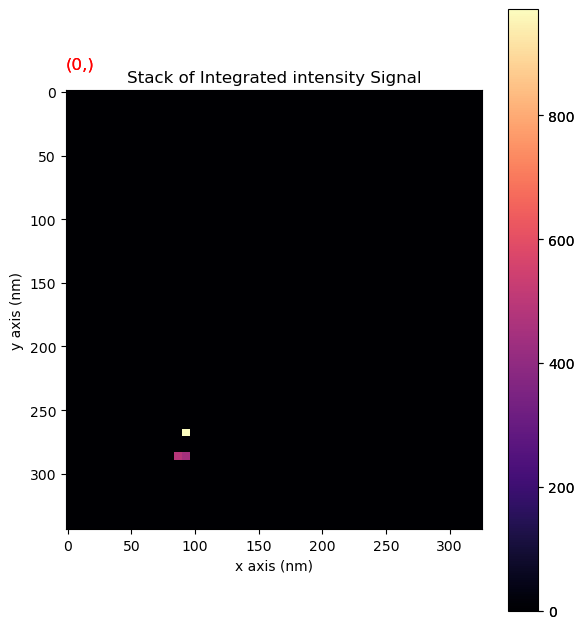
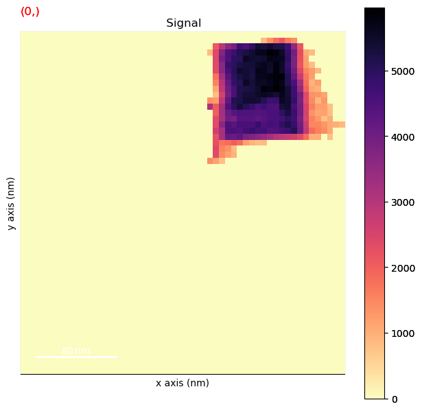
Plot the VDF images for inspection

[ ]:

#%matplotlib notebook
VDFs.plot(cmap='magma', scalebar=False)

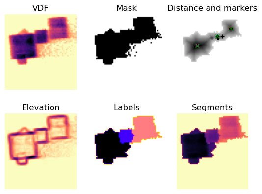
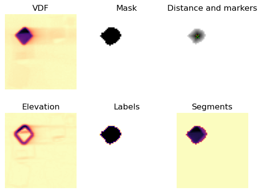
../../_images/tutorials_pyxem-demos_06_Nanocrystal_segmentation_in_SPED_data_-_Demonstration_on_partly_overlapping_MgO_cubes_71_0.png

../../_images/tutorials_pyxem-demos_06_Nanocrystal_segmentation_in_SPED_data_-_Demonstration_on_partly_overlapping_MgO_cubes_71_1.png

First find adequate parameters by looking at watershed segmentation of a single VDF image.

[ ]:

from pyxem.utils.segment_utils import separate_watershed

[ ]:

min_distance = 5.5
min_size = 10
max_size = 1000
max_number_of_grains = 1000
marker_radius = 2
exclude_border = 2

[ ]:

i = 3
sep_i = separate_watershed(
    VDFs.inav[i].data, min_distance=min_distance, min_size=min_size,
    max_size=max_size, max_number_of_grains=max_number_of_grains,
    exclude_border=exclude_border, marker_radius=marker_radius,
    threshold=True, plot_on=True)

../../_images/tutorials_pyxem-demos_06_Nanocrystal_segmentation_in_SPED_data_-_Demonstration_on_partly_overlapping_MgO_cubes_75_0.png

Perform segmentation on all the VDF images

[ ]:

segs = VDFs.get_vdf_segments(min_distance=min_distance,
                             min_size=min_size,
                             max_size = max_size,
                             max_number_of_grains = max_number_of_grains,
                             exclude_border=exclude_border,
                             marker_radius=marker_radius,
                             threshold=True)

print(np.shape(segs.segments)[0],' segments were found.')

[                                        ] | 0% Completed | 103.46 ms

/home/cssfrancis/hyperspy-bundle/lib/python3.10/site-packages/pyxem/signals/virtual_dark_field_image.py:110: UserWarning: Changed in version 0.15.0.  May cause unexpectederrors related to managing the proper axes.
  warnings.warn(
/home/cssfrancis/hyperspy-bundle/lib/python3.10/site-packages/skimage/filters/thresholding.py:757: RuntimeWarning: divide by zero encountered in log
  / (np.log(mean_back) - np.log(mean_fore)))
/home/cssfrancis/hyperspy-bundle/lib/python3.10/site-packages/skimage/filters/thresholding.py:757: RuntimeWarning: divide by zero encountered in log
  / (np.log(mean_back) - np.log(mean_fore)))
/home/cssfrancis/hyperspy-bundle/lib/python3.10/site-packages/skimage/filters/thresholding.py:757: RuntimeWarning: divide by zero encountered in log
  / (np.log(mean_back) - np.log(mean_fore)))
/home/cssfrancis/hyperspy-bundle/lib/python3.10/site-packages/skimage/filters/thresholding.py:757: RuntimeWarning: divide by zero encountered in log
  / (np.log(mean_back) - np.log(mean_fore)))

[########################################] | 100% Completed | 204.43 ms
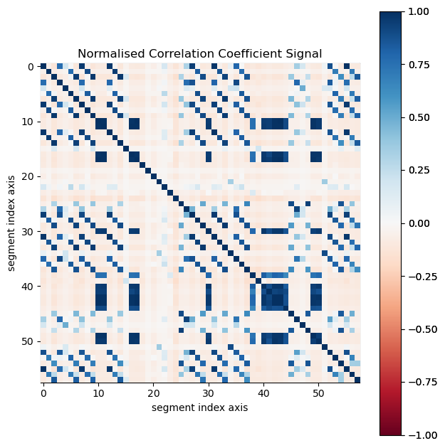
58  segments were found.

Plot the segments for inspection

[ ]:

segs.segments.plot(cmap='magma_r')

../../_images/tutorials_pyxem-demos_06_Nanocrystal_segmentation_in_SPED_data_-_Demonstration_on_partly_overlapping_MgO_cubes_79_0.png

../../_images/tutorials_pyxem-demos_06_Nanocrystal_segmentation_in_SPED_data_-_Demonstration_on_partly_overlapping_MgO_cubes_79_1.png

Calculate normalised cross-correlations between all VDF image segments to identify those that are related to the same crystal.

[ ]:

ncc_vdf = segs.get_ncc_matrix()
ncc_vdf.plot(scalebar=False, cmap='RdBu')

../../_images/tutorials_pyxem-demos_06_Nanocrystal_segmentation_in_SPED_data_-_Demonstration_on_partly_overlapping_MgO_cubes_81_0.png

If the correlation value exceeds corr_threshold for certain segments, those segments are summed. These segments are discarded if the number of these segments are below vector_threshold, as this number corresponds to the number of detected diffraction peaks associated with the single crystal. The vector_threshold criteria is included to avoid including segment images resulting from noise or incorrect segmentation.

[ ]:

corr_threshold=0.3
vector_threshold=5
segment_threshold=3

[ ]:

corrsegs = segs.correlate_vdf_segments(
    corr_threshold=corr_threshold, vector_threshold=vector_threshold,
    segment_threshold=segment_threshold)
print(np.shape(corrsegs.segments)[0],' correlated segments were found.')

  0%|                                                                                                   | 0/58 [00:00<?, ?it/s]

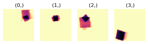
4  correlated segments were found.

Simulate virtual diffraction patterns for each summed segment

[ ]:

sigma = scale*1.5

virtual_sig = corrsegs.get_virtual_electron_diffraction(
    calibration=scale, shape=(int(radius_px*2), int(radius_px*2)), sigma=sigma)
virtual_sig.set_diffraction_calibration(scale)

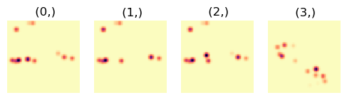
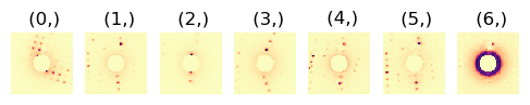
Plot the final results from the VDF image-based segmentation

[ ]:

hs.plot.plot_images(corrsegs.segments, cmap='magma_r', axes_decor='off',
                    per_row=np.shape(corrsegs.segments)[0],
                    suptitle='', scalebar=False, scalebar_color='white',
                    colorbar=False,
                    padding={'top': 0.95, 'bottom': 0.05,
                             'left': 0.05, 'right':0.78})

[<Axes: title={'center': ' (0,)'}, xlabel='x axis (nm)', ylabel='y axis (nm)'>,
 <Axes: title={'center': ' (1,)'}, xlabel='x axis (nm)', ylabel='y axis (nm)'>,
 <Axes: title={'center': ' (2,)'}, xlabel='x axis (nm)', ylabel='y axis (nm)'>,
 <Axes: title={'center': ' (3,)'}, xlabel='x axis (nm)', ylabel='y axis (nm)'>]

../../_images/tutorials_pyxem-demos_06_Nanocrystal_segmentation_in_SPED_data_-_Demonstration_on_partly_overlapping_MgO_cubes_88_1.png

[ ]:

hs.plot.plot_images(virtual_sig, cmap='magma_r', axes_decor='off',
                    per_row=np.shape(corrsegs.segments)[0],
                    suptitle='', scalebar=False, scalebar_color='white',
                    colorbar=False,
                    padding={'top': 0.95, 'bottom': 0.05,
                             'left': 0.05, 'right': 0.78})

[<Axes: title={'center': ' (0,)'}, xlabel='kx axis ($A^{-1}$)', ylabel='ky axis ($A^{-1}$)'>,
 <Axes: title={'center': ' (1,)'}, xlabel='kx axis ($A^{-1}$)', ylabel='ky axis ($A^{-1}$)'>,
 <Axes: title={'center': ' (2,)'}, xlabel='kx axis ($A^{-1}$)', ylabel='ky axis ($A^{-1}$)'>,
 <Axes: title={'center': ' (3,)'}, xlabel='kx axis ($A^{-1}$)', ylabel='ky axis ($A^{-1}$)'>]

../../_images/tutorials_pyxem-demos_06_Nanocrystal_segmentation_in_SPED_data_-_Demonstration_on_partly_overlapping_MgO_cubes_89_1.png

3. NMF Based Segmentation#

3.1. NMF Decomposition#

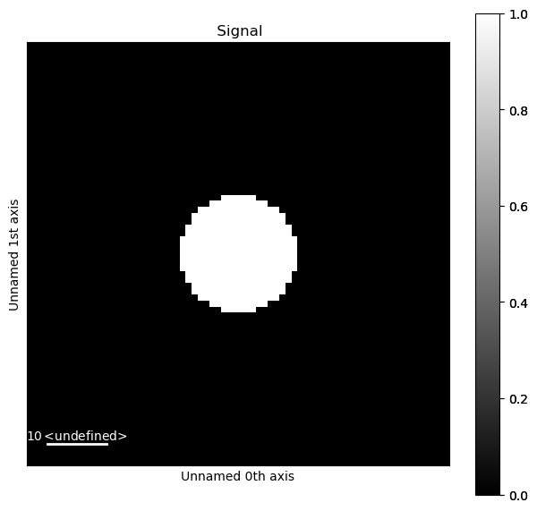
Create a signal mask so that the region in the centre of each PED pattern, including the direct beam, can be excluded in the machine learning.

[ ]:

dpm = pxm.signals.Diffraction2D(dp.inav[0,0])
signal_mask = dpm.get_direct_beam_mask(radius=10)
signal_mask.plot()

../../_images/tutorials_pyxem-demos_06_Nanocrystal_segmentation_in_SPED_data_-_Demonstration_on_partly_overlapping_MgO_cubes_94_0.png

Perform single value decomposition (SVD)

[ ]:

dp.change_dtype('float32')
dp.decomposition(algorithm='SVD',
                 normalize_poissonian_noise=True,
                 centre=None,
                 signal_mask=signal_mask.data)

Decomposition info:
  normalize_poissonian_noise=True
  algorithm=SVD
  output_dimension=None
  centre=None

[ ]:

dp.plot_decomposition_results()

WARNING:hyperspy_gui_traitsui:The module://matplotlib_inline.backend_inline matplotlib backend is not compatible with the traitsui GUI elements. For more information, read http://hyperspy.readthedocs.io/en/stable/user_guide/getting_started.html#possible-warnings-when-importing-hyperspy.

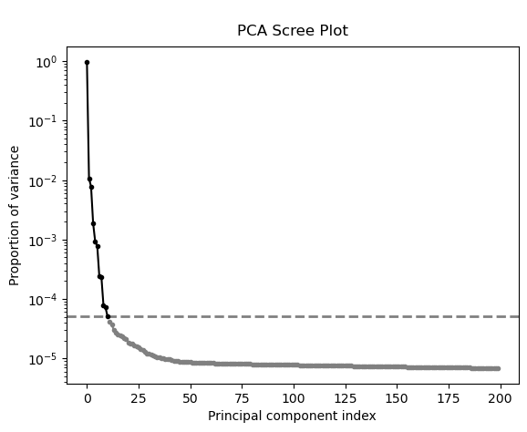
../../_images/tutorials_pyxem-demos_06_Nanocrystal_segmentation_in_SPED_data_-_Demonstration_on_partly_overlapping_MgO_cubes_97_2.png

../../_images/tutorials_pyxem-demos_06_Nanocrystal_segmentation_in_SPED_data_-_Demonstration_on_partly_overlapping_MgO_cubes_97_3.png

Investigate the scree plot and use it as a guide to determine the number of components

[ ]:

num_comp=11

ax = dp.plot_explained_variance_ratio(n=200, threshold=num_comp,
                                      hline=True, xaxis_labeling='ordinal',
                                      signal_fmt={'color':'k', 'marker':'.'},
                                      noise_fmt={'color':'gray', 'marker':'.'})

../../_images/tutorials_pyxem-demos_06_Nanocrystal_segmentation_in_SPED_data_-_Demonstration_on_partly_overlapping_MgO_cubes_99_0.png

Perform NMF decomposition with specified number of components

[ ]:

dp.decomposition(normalize_poissonian_noise=True,
                 algorithm='NMF',
                 output_dimension=num_comp,
                 signal_mask=signal_mask.data)

Decomposition info:
  normalize_poissonian_noise=True
  algorithm=NMF
  output_dimension=11
  centre=None
scikit-learn estimator:
NMF(n_components=11)

/home/cssfrancis/hyperspy-bundle/lib/python3.10/site-packages/sklearn/decomposition/_nmf.py:1665: ConvergenceWarning: Maximum number of iterations 200 reached. Increase it to improve convergence.
  warnings.warn(

[ ]:

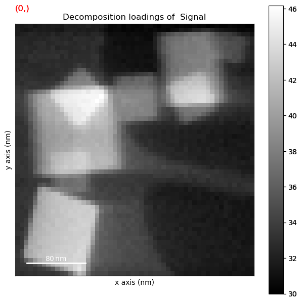
dp_nmf = dp.get_decomposition_model(components=np.arange(num_comp))
factors = dp_nmf.get_decomposition_factors()
loadings = dp_nmf.get_decomposition_loadings()

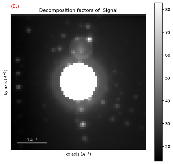
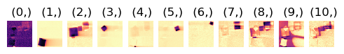
Plot the NMF results

[ ]:

hs.plot.plot_images(loadings, cmap='magma_r', axes_decor='off', per_row=11,
             suptitle='', scalebar=False, scalebar_color='white', colorbar=False,
             padding={'top': 0.95, 'bottom': 0.05,
                      'left': 0.05, 'right':0.78})
hs.plot.plot_images(factors, cmap='magma_r', axes_decor='off', per_row=11,
             suptitle='', scalebar=False, scalebar_color='white', colorbar=False,
             padding={'top': 0.95, 'bottom': 0.05,
                      'left': 0.05, 'right':0.78})

[<Axes: title={'center': ' (0,)'}, xlabel='kx axis ($A^{-1}$)', ylabel='ky axis ($A^{-1}$)'>,
 <Axes: title={'center': ' (1,)'}, xlabel='kx axis ($A^{-1}$)', ylabel='ky axis ($A^{-1}$)'>,
 <Axes: title={'center': ' (2,)'}, xlabel='kx axis ($A^{-1}$)', ylabel='ky axis ($A^{-1}$)'>,
 <Axes: title={'center': ' (3,)'}, xlabel='kx axis ($A^{-1}$)', ylabel='ky axis ($A^{-1}$)'>,
 <Axes: title={'center': ' (4,)'}, xlabel='kx axis ($A^{-1}$)', ylabel='ky axis ($A^{-1}$)'>,
 <Axes: title={'center': ' (5,)'}, xlabel='kx axis ($A^{-1}$)', ylabel='ky axis ($A^{-1}$)'>,
 <Axes: title={'center': ' (6,)'}, xlabel='kx axis ($A^{-1}$)', ylabel='ky axis ($A^{-1}$)'>,
 <Axes: title={'center': ' (7,)'}, xlabel='kx axis ($A^{-1}$)', ylabel='ky axis ($A^{-1}$)'>,
 <Axes: title={'center': ' (8,)'}, xlabel='kx axis ($A^{-1}$)', ylabel='ky axis ($A^{-1}$)'>,
 <Axes: title={'center': ' (9,)'}, xlabel='kx axis ($A^{-1}$)', ylabel='ky axis ($A^{-1}$)'>,
 <Axes: title={'center': ' (10,)'}, xlabel='kx axis ($A^{-1}$)', ylabel='ky axis ($A^{-1}$)'>]

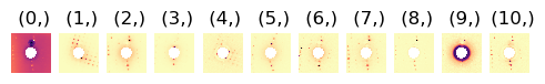
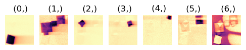
../../_images/tutorials_pyxem-demos_06_Nanocrystal_segmentation_in_SPED_data_-_Demonstration_on_partly_overlapping_MgO_cubes_104_1.png

../../_images/tutorials_pyxem-demos_06_Nanocrystal_segmentation_in_SPED_data_-_Demonstration_on_partly_overlapping_MgO_cubes_104_2.png

Discard the components related to background (#0) and to the carbon film (#4)

[ ]:

from hyperspy.signals import Signal2D

[ ]:

factors = Signal2D(np.delete(factors.data, [0, 4], axis = 0))
loadings = Signal2D(np.delete(loadings.data, [0, 4], axis = 0))

[ ]:

hs.plot.plot_images(factors, cmap='magma_r', axes_decor='off',
                    per_row=9, suptitle='', scalebar=False,
                    scalebar_color='white', colorbar=False,
                    padding={'top': 0.95, 'bottom': 0.05,
                             'left': 0.05, 'right':0.78})

hs.plot.plot_images(loadings, cmap='magma_r', axes_decor='off',
                    per_row=9, suptitle='', scalebar=False,
                    scalebar_color='white', colorbar=False,
                    padding={'top': 0.95, 'bottom': 0.05,
                             'left': 0.05, 'right':0.78})

[<Axes: title={'center': ' (0,)'}>,
 <Axes: title={'center': ' (1,)'}>,
 <Axes: title={'center': ' (2,)'}>,
 <Axes: title={'center': ' (3,)'}>,
 <Axes: title={'center': ' (4,)'}>,
 <Axes: title={'center': ' (5,)'}>,
 <Axes: title={'center': ' (6,)'}>,
 <Axes: title={'center': ' (7,)'}>,
 <Axes: title={'center': ' (8,)'}>]

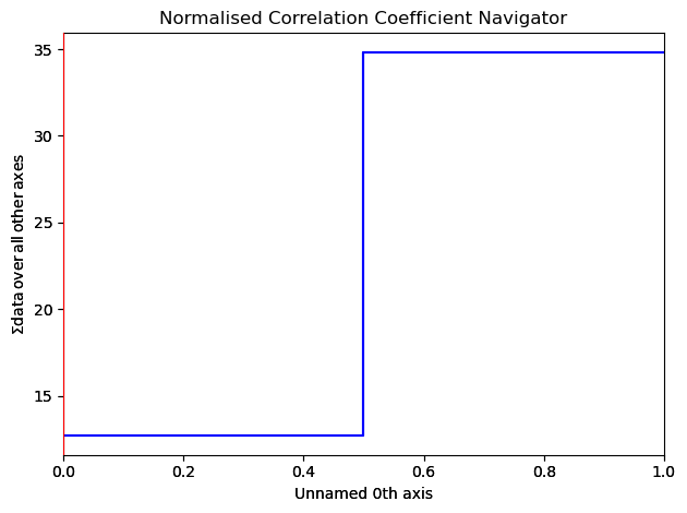
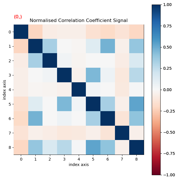
../../_images/tutorials_pyxem-demos_06_Nanocrystal_segmentation_in_SPED_data_-_Demonstration_on_partly_overlapping_MgO_cubes_108_1.png

../../_images/tutorials_pyxem-demos_06_Nanocrystal_segmentation_in_SPED_data_-_Demonstration_on_partly_overlapping_MgO_cubes_108_2.png

3.2. Correlate NMF Loading Maps#

NMF often leads to splitting of some crystals into several components. Therefore the correlation between loadings and between component patterns are calculated, and if both the correlation values for loadings and factors exceed threshold values, those loadings and factors are summed.

Calculate the matrix of normalised cross-correlation for both the loadings and patterns first, to find suitable correlation threshold values.

[ ]:

from pyxem.signals.segments import LearningSegment
learn = LearningSegment(factors=factors, loadings=loadings)

[ ]:

ncc_nmf = learn.get_ncc_matrix()

[########################################] | 100% Completed | 102.58 ms
[########################################] | 100% Completed | 101.97 ms

[ ]:

ncc_nmf.plot(scalebar=False, cmap='RdBu')

../../_images/tutorials_pyxem-demos_06_Nanocrystal_segmentation_in_SPED_data_-_Demonstration_on_partly_overlapping_MgO_cubes_114_0.png

../../_images/tutorials_pyxem-demos_06_Nanocrystal_segmentation_in_SPED_data_-_Demonstration_on_partly_overlapping_MgO_cubes_114_1.png

[ ]:

corr_th_factors = 0.45
corr_th_loadings = 0.3

Perform correlation and summation of the factors and loadings

[ ]:

learn_corr = learn.correlate_learning_segments(corr_th_factors=corr_th_factors,
                                               corr_th_loadings=corr_th_loadings)

[########################################] | 100% Completed | 101.88 ms
[########################################] | 100% Completed | 102.38 ms

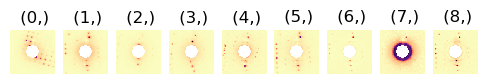
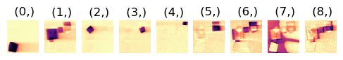
Plot the NMF reuslts after correlation and summation

[ ]:

hs.plot.plot_images(learn_corr.loadings, cmap='magma_r', axes_decor='off',
                    per_row=7, suptitle='', scalebar=False,
                    scalebar_color='white', colorbar=False,
                    padding={'top': 0.95, 'bottom': 0.05,
                             'left': 0.05, 'right':0.78})
hs.plot.plot_images(learn_corr.factors, cmap='magma_r', axes_decor='off',
                    per_row=7, suptitle='', scalebar=False,
                    scalebar_color='white', colorbar=False,
                    padding={'top': 0.95, 'bottom': 0.05,
                             'left': 0.05, 'right':0.78})

[<Axes: title={'center': ' (0,)'}>,
 <Axes: title={'center': ' (1,)'}>,
 <Axes: title={'center': ' (2,)'}>,
 <Axes: title={'center': ' (3,)'}>,
 <Axes: title={'center': ' (4,)'}>,
 <Axes: title={'center': ' (5,)'}>,
 <Axes: title={'center': ' (6,)'}>]

../../_images/tutorials_pyxem-demos_06_Nanocrystal_segmentation_in_SPED_data_-_Demonstration_on_partly_overlapping_MgO_cubes_119_1.png

../../_images/tutorials_pyxem-demos_06_Nanocrystal_segmentation_in_SPED_data_-_Demonstration_on_partly_overlapping_MgO_cubes_119_2.png

First investigate how the parameters influence the segmentation on one single loading map.

[ ]:

from pyxem.utils.segment_utils import separate_watershed

[ ]:

min_distance = 10
min_size = 50
max_size = 100000
max_number_of_grains = 100000
marker_radius = 2
exclude_border = 1
threshold = True

[ ]:

i =2
sep_i = separate_watershed(
    learn_corr.loadings.data[i], min_distance=min_distance,
    min_size=min_size, max_size=max_size,
    max_number_of_grains=max_number_of_grains,
    exclude_border=exclude_border,
    marker_radius=marker_radius, threshold=True, plot_on=True)

../../_images/tutorials_pyxem-demos_06_Nanocrystal_segmentation_in_SPED_data_-_Demonstration_on_partly_overlapping_MgO_cubes_123_0.png

Set a threshold for the minimum intensity value that a loading segment must contain in order to be kept.

[ ]:

min_intensity_threshold = 10000

[ ]:

learn_corr_seg = learn_corr.separate_learning_segments(
    min_intensity_threshold=min_intensity_threshold,
    min_distance = min_distance, min_size = min_size,
    max_size = max_size,
    max_number_of_grains = max_number_of_grains,
    exclude_border = exclude_border,
    marker_radius = marker_radius, threshold = True)

[########################################] | 100% Completed | 101.13 ms

Plot the final results from the NMF-based segmentation

[ ]:

learn_corr_seg.loadings

<Signal2D, title: , dimensions: (0|54, 57)>

[ ]:

hs.plot.plot_images(learn_corr_seg.loadings,
                    cmap='magma_r', axes_decor='off',
                    per_row=10, suptitle='', scalebar=False,
                    scalebar_color='white', colorbar=False,
                    padding={'top': 0.95, 'bottom': 0.05,
                             'left': 0.05, 'right':0.78})

hs.plot.plot_images(learn_corr_seg.factors,
                    cmap='magma_r', axes_decor='off',
                    per_row=10, suptitle='', scalebar=False,
                    scalebar_color='white', colorbar=False,
                    padding={'top': 0.95, 'bottom': 0.05,
                             'left': 0.05, 'right':0.78})
plt.show()

<Figure size 640x640 with 0 Axes>

<Figure size 640x640 with 0 Axes>