Creating a Segmented Detector

In this example we will show how to create virtual images for a segmented-like detector.

This is helpful for basic mapping of orientation etc. in a diffraction pattern and can be useful for a first look at the data.

import pyxem as pxm
from pyxem.utils._azimuthal_integrations import _get_control_points
import numpy as np
import hyperspy.api as hs


dp = pxm.data.tilt_boundary_data()
dp.calibrate.center = None  # Center the diffraction patterns
dp.calibrate.scale = 0.1  # Scale the diffraction patterns in reciprocal space


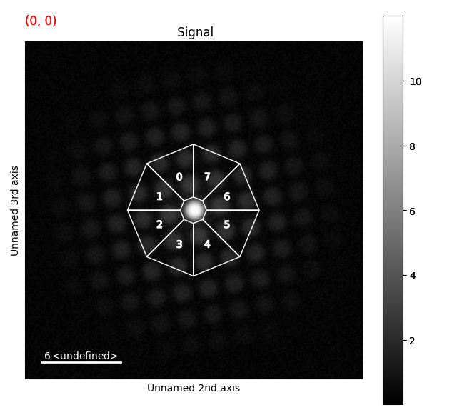
# Visualizing the virtual detector
cp = _get_control_points(
    1,
    npt_azim=8,
    radial_range=(1, 5),
    azimuthal_range=(-np.pi, np.pi),
    affine=dp.calibrate.affine,
)[:, :, ::-1]
poly = hs.plot.markers.Polygons(verts=cp, edgecolor="w", facecolor="none")
dp.plot()
dp.add_marker(poly)
pos = np.mean(cp, axis=1)
texts = np.arange(len(pos)).astype(str)
texts = hs.plot.markers.Texts(offsets=pos, texts=texts, color="w")
dp.add_marker(texts)

• 
• 

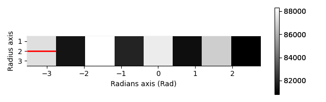
az = dp.get_azimuthal_integral2d(npt=1, npt_azim=8, radial_range=(2, 5))

az.T.plot()

• 
• 

[                                        ] | 0% Completed | 150.74 us
[########################################] | 100% Completed | 100.50 ms

sphinx_gallery_thumbnail_number = 2 %%