Background subtraction

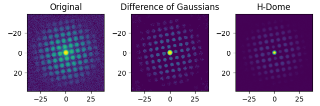
If your diffraction data is noisy, you might want to subtract the background from the dataset. Pyxem offers some built-in functionality for this, with the subtract_diffraction_background class method. Custom filtering is also possible, an example is shown in the ‘Filtering Data’-example.

import pyxem as pxm
import hyperspy.api as hs

s = pxm.data.tilt_boundary_data()

s_filtered = s.subtract_diffraction_background(
    "difference of gaussians",
    inplace=False,
    min_sigma=3,
    max_sigma=20,
)

s_filtered_h = s.subtract_diffraction_background("h-dome", inplace=False, h=0.7)


hs.plot.plot_images(
    [s.inav[2, 2], s_filtered.inav[2, 2], s_filtered_h.inav[2, 2]],
    label=["Original", "Difference of Gaussians", "H-Dome"],
    tight_layout=True,
    norm="symlog",
    cmap="viridis",
    colorbar=None,
)

[                                        ] | 0% Completed | 137.39 us
[                                        ] | 0% Completed | 100.92 ms
[                                        ] | 0% Completed | 201.25 ms
[                                        ] | 0% Completed | 301.64 ms
[                                        ] | 0% Completed | 402.01 ms
[                                        ] | 0% Completed | 502.36 ms
[                                        ] | 0% Completed | 602.89 ms
[                                        ] | 0% Completed | 703.24 ms
[                                        ] | 0% Completed | 803.60 ms
[                                        ] | 0% Completed | 903.96 ms
[                                        ] | 0% Completed | 1.00 s
[                                        ] | 0% Completed | 1.10 s
[                                        ] | 0% Completed | 1.21 s
[                                        ] | 0% Completed | 1.31 s
[                                        ] | 0% Completed | 1.41 s
[########################################] | 100% Completed | 1.51 s
/home/docs/checkouts/readthedocs.org/user_builds/pyxem/envs/latest/lib/python3.10/site-packages/hyperspy/misc/utils.py:1434: UserWarning: Possible precision loss converting image of type float32 to uint8 as required by rank filters. Convert manually using skimage.util.img_as_ubyte to silence this warning.
  output = function(test_data, **kwargs)

[                                        ] | 0% Completed | 137.55 us/home/docs/checkouts/readthedocs.org/user_builds/pyxem/envs/latest/lib/python3.10/site-packages/hyperspy/misc/utils.py:1357: UserWarning: Possible precision loss converting image of type float32 to uint8 as required by rank filters. Convert manually using skimage.util.img_as_ubyte to silence this warning.
  output_array[islice] = function(data[islice], **kwargs)

[                                        ] | 0% Completed | 100.41 ms
[                                        ] | 0% Completed | 200.77 ms
[                                        ] | 0% Completed | 301.09 ms
[                                        ] | 0% Completed | 401.63 ms
[                                        ] | 0% Completed | 502.02 ms
[                                        ] | 0% Completed | 602.42 ms
[                                        ] | 0% Completed | 702.76 ms
[                                        ] | 0% Completed | 803.14 ms
[                                        ] | 0% Completed | 903.53 ms
[                                        ] | 0% Completed | 1.00 s
[                                        ] | 0% Completed | 1.10 s
[                                        ] | 0% Completed | 1.20 s
[                                        ] | 0% Completed | 1.30 s
[                                        ] | 0% Completed | 1.41 s
[                                        ] | 0% Completed | 1.51 s
[                                        ] | 0% Completed | 1.61 s
[                                        ] | 0% Completed | 1.71 s
[                                        ] | 0% Completed | 1.81 s
[                                        ] | 0% Completed | 1.91 s
[                                        ] | 0% Completed | 2.01 s
[                                        ] | 0% Completed | 2.11 s
[                                        ] | 0% Completed | 2.21 s
[                                        ] | 0% Completed | 2.31 s
[                                        ] | 0% Completed | 2.41 s
[                                        ] | 0% Completed | 2.51 s
[                                        ] | 0% Completed | 2.61 s
[                                        ] | 0% Completed | 2.71 s
[########################################] | 100% Completed | 2.81 s

[<Axes: title={'center': 'Original'}>, <Axes: title={'center': 'Difference of Gaussians'}>, <Axes: title={'center': 'H-Dome'}>]

Filtering Polar Images

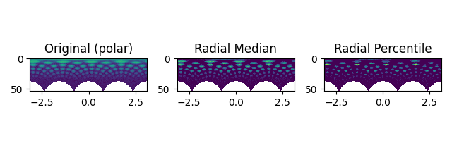
The available methods differ for Diffraction2D datasets and PolarDiffraction2D datasets.

Set the center of the diffraction pattern to its default, i.e. the middle of the image

s.calibrate.center = None

Transform to polar coordinates

s_polar = s.get_azimuthal_integral2d(npt=100, mean=True)

s_polar_filtered = s_polar.subtract_diffraction_background(
    "radial median",
    inplace=False,
)

s_polar_filtered2 = s_polar.subtract_diffraction_background(
    "radial percentile",
    percentile=70,
    inplace=False,
)

hs.plot.plot_images(
    [s_polar.inav[2, 2], s_polar_filtered.inav[2, 2], s_polar_filtered2.inav[2, 2]],
    label=["Original (polar)", "Radial Median", "Radial Percentile"],
    tight_layout=True,
    norm="symlog",
    cmap="viridis",
    colorbar=None,
)

[                                        ] | 0% Completed | 154.75 us
[                                        ] | 0% Completed | 100.48 ms
[                                        ] | 0% Completed | 200.85 ms
[                                        ] | 0% Completed | 301.19 ms
[                                        ] | 0% Completed | 401.57 ms
[                                        ] | 0% Completed | 501.93 ms
[                                        ] | 0% Completed | 602.70 ms
[########################################] | 100% Completed | 703.28 ms

[                                        ] | 0% Completed | 143.10 us
[                                        ] | 0% Completed | 100.48 ms
[########################################] | 100% Completed | 200.88 ms

[                                        ] | 0% Completed | 137.85 us
[                                        ] | 0% Completed | 100.52 ms
[                                        ] | 0% Completed | 200.86 ms
[                                        ] | 0% Completed | 301.30 ms
[                                        ] | 0% Completed | 401.62 ms
[                                        ] | 0% Completed | 502.08 ms
[                                        ] | 0% Completed | 602.44 ms
[                                        ] | 0% Completed | 702.80 ms
[                                        ] | 0% Completed | 803.15 ms
[                                        ] | 0% Completed | 903.49 ms
[########################################] | 100% Completed | 1.00 s

[<Axes: title={'center': 'Original (polar)'}>, <Axes: title={'center': 'Radial Median'}>, <Axes: title={'center': 'Radial Percentile'}>]