Strain Mapping

Strain mapping in pyxem is done by fitting a DisplacementGradientMap to the data. This can be thought of as image distortion around some central point.

from pyxem.data import simulated_strain
import hyperspy.api as hs

In this example we will create a simulated strain map using the simulated_strain() function. This just creates a simulated diffraction pattern and applies a simple “strain” to it. In this case using simulated data is slightly easier for demonstration purposes. If you want to use real data the zrnb_precipitate() dataset is a good example of strain from a precipitate.

strained_signal = simulated_strain(
    navigation_shape=(32, 32),
    signal_shape=(512, 512),
    disk_radius=20,
    num_electrons=1e5,
    strain_matrix=None,
    lazy=True,
)

The first thing we want to do is to find peaks within the diffraction pattern. I’d recommend using the get_diffraction_vectors() method

strained_signal.calibration.center = (
    None  # First set the center to be (256, 256) or the center of the signal
)
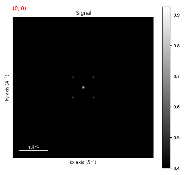
template_matched = strained_signal.template_match_disk(disk_r=20, subtract_min=False)
template_matched.plot(vmin=0.4)

• 
• 

  0%|          | 0/65 [00:00<?, ?it/s]
  2%|▏         | 1/65 [00:00<01:00,  1.06it/s]
  8%|▊         | 5/65 [00:01<00:20,  2.97it/s]
 11%|█         | 7/65 [00:02<00:14,  4.04it/s]
 14%|█▍        | 9/65 [00:02<00:16,  3.36it/s]
 17%|█▋        | 11/65 [00:03<00:12,  4.18it/s]
 20%|██        | 13/65 [00:03<00:14,  3.61it/s]
 23%|██▎       | 15/65 [00:04<00:11,  4.22it/s]
 26%|██▌       | 17/65 [00:04<00:12,  3.77it/s]
 29%|██▉       | 19/65 [00:05<00:10,  4.36it/s]
 32%|███▏      | 21/65 [00:05<00:11,  3.96it/s]
 35%|███▌      | 23/65 [00:05<00:09,  4.43it/s]
 38%|███▊      | 25/65 [00:06<00:09,  4.27it/s]
 42%|████▏     | 27/65 [00:06<00:08,  4.37it/s]
 45%|████▍     | 29/65 [00:07<00:08,  4.37it/s]
 48%|████▊     | 31/65 [00:07<00:07,  4.33it/s]
 51%|█████     | 33/65 [00:08<00:07,  4.47it/s]
 54%|█████▍    | 35/65 [00:08<00:07,  4.25it/s]
 57%|█████▋    | 37/65 [00:09<00:06,  4.54it/s]
 60%|██████    | 39/65 [00:09<00:06,  4.17it/s]
 63%|██████▎   | 41/65 [00:10<00:05,  4.66it/s]
 66%|██████▌   | 43/65 [00:10<00:05,  4.11it/s]
 69%|██████▉   | 45/65 [00:10<00:04,  4.93it/s]
 72%|███████▏  | 47/65 [00:11<00:04,  4.01it/s]
 75%|███████▌  | 49/65 [00:11<00:03,  5.00it/s]
 78%|███████▊  | 51/65 [00:12<00:03,  4.09it/s]
 82%|████████▏ | 53/65 [00:12<00:02,  4.95it/s]
 85%|████████▍ | 55/65 [00:13<00:02,  4.01it/s]
 88%|████████▊ | 57/65 [00:13<00:01,  5.02it/s]
 91%|█████████ | 59/65 [00:14<00:01,  3.91it/s]
 97%|█████████▋| 63/65 [00:14<00:00,  5.26it/s]
100%|██████████| 65/65 [00:14<00:00,  4.39it/s]

Plotting the template matched signal and setting vmin is a good way to see what threshold you should use for the get_diffraction_vectors() method.

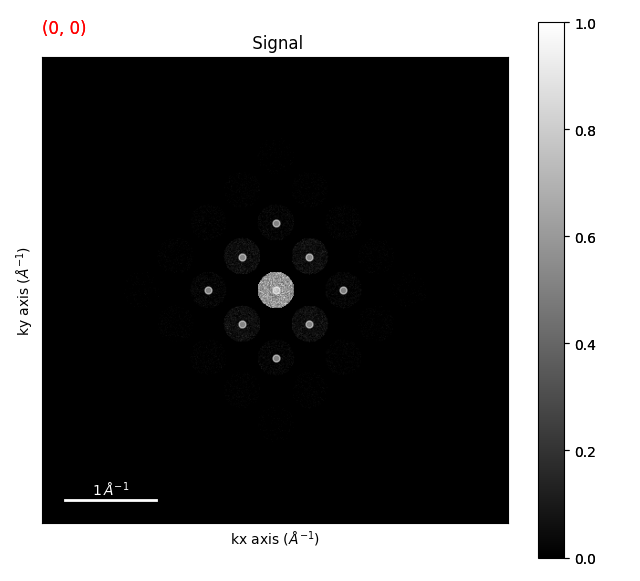
diffraction_vectors = template_matched.get_diffraction_vectors(
    threshold_abs=0.4, min_distance=5
)

markers = diffraction_vectors.to_markers(color="w", sizes=5, alpha=0.5)
strained_signal.plot()
strained_signal.add_marker(markers)

• 
• 

  0%|          | 0/65 [00:00<?, ?it/s]
100%|██████████| 65/65 [00:00<00:00, 763.54it/s]

Determining the Strain

We can just use the first ring of the diffraction pattern to determine the strain. We can do this by using the filter_magnitude() method. You can also look at the filtering vectors example to see how to select which vectors you want to use more generally. You can also just manually input the un-strained vectors or use simulated/ rotated vectors as well.

first_ring_vectors = diffraction_vectors.filter_magnitude(
    min_magnitude=0.1,
    max_magnitude=1,
)
unstrained_vectors = first_ring_vectors.inav[0, 0]

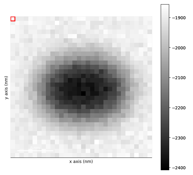
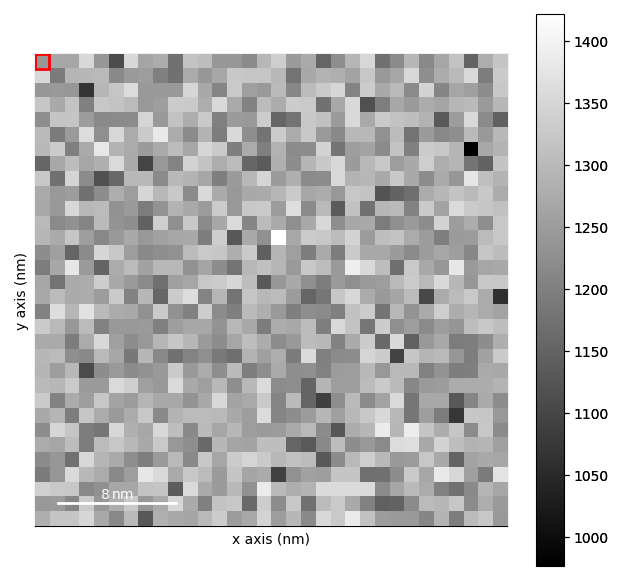
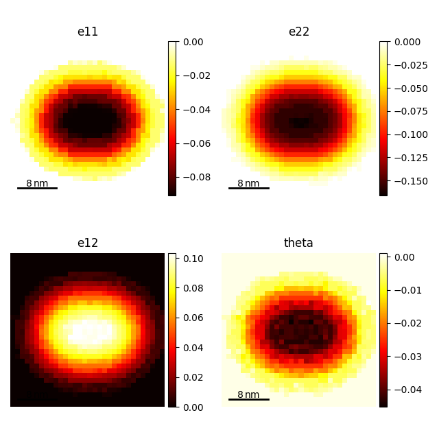
strain_maps = first_ring_vectors.get_strain_maps(
    unstrained_vectors=unstrained_vectors, return_residuals=False
)

strain_maps.plot()

  0%|          | 0/2 [00:00<?, ?it/s]
 50%|█████     | 1/2 [00:00<00:00,  1.60it/s]
100%|██████████| 2/2 [00:00<00:00,  3.21it/s]

  0%|          | 0/65 [00:00<?, ?it/s]
  2%|▏         | 1/65 [00:01<01:20,  1.26s/it]
  8%|▊         | 5/65 [00:02<00:27,  2.15it/s]
 14%|█▍        | 9/65 [00:03<00:21,  2.58it/s]
 20%|██        | 13/65 [00:05<00:18,  2.80it/s]
 23%|██▎       | 15/65 [00:05<00:14,  3.47it/s]
 26%|██▌       | 17/65 [00:06<00:17,  2.80it/s]
 29%|██▉       | 19/65 [00:06<00:13,  3.37it/s]
 32%|███▏      | 21/65 [00:07<00:15,  2.82it/s]
 35%|███▌      | 23/65 [00:07<00:12,  3.33it/s]
 38%|███▊      | 25/65 [00:08<00:14,  2.83it/s]
 42%|████▏     | 27/65 [00:09<00:11,  3.30it/s]
 45%|████▍     | 29/65 [00:10<00:12,  2.84it/s]
 48%|████▊     | 31/65 [00:10<00:10,  3.33it/s]
 51%|█████     | 33/65 [00:11<00:11,  2.85it/s]
 54%|█████▍    | 35/65 [00:11<00:09,  3.26it/s]
 57%|█████▋    | 37/65 [00:12<00:09,  2.86it/s]
 60%|██████    | 39/65 [00:13<00:07,  3.27it/s]
 63%|██████▎   | 41/65 [00:14<00:08,  2.94it/s]
 66%|██████▌   | 43/65 [00:14<00:06,  3.17it/s]
 69%|██████▉   | 45/65 [00:15<00:06,  2.96it/s]
 72%|███████▏  | 47/65 [00:15<00:05,  3.13it/s]
 75%|███████▌  | 49/65 [00:16<00:05,  2.97it/s]
 78%|███████▊  | 51/65 [00:17<00:04,  3.04it/s]
 82%|████████▏ | 53/65 [00:18<00:04,  2.99it/s]
 85%|████████▍ | 55/65 [00:18<00:03,  3.01it/s]
 88%|████████▊ | 57/65 [00:19<00:02,  3.03it/s]
 91%|█████████ | 59/65 [00:20<00:02,  2.96it/s]
 94%|█████████▍| 61/65 [00:20<00:01,  3.13it/s]
 97%|█████████▋| 63/65 [00:20<00:00,  3.62it/s]
100%|██████████| 65/65 [00:20<00:00,  3.10it/s]

  0%|          | 0/33 [00:00<?, ?it/s]
100%|██████████| 33/33 [00:00<00:00, 1173.76it/s]

  0%|          | 0/33 [00:00<?, ?it/s]
100%|██████████| 33/33 [00:00<00:00, 1738.76it/s]

  0%|          | 0/33 [00:00<?, ?it/s]
100%|██████████| 33/33 [00:00<00:00, 7502.41it/s]

  0%|          | 0/9 [00:00<?, ?it/s]
100%|██████████| 9/9 [00:00<00:00, 11308.79it/s]

[<Axes: title={'center': 'e11'}, xlabel='x axis (nm)', ylabel='y axis (nm)'>, <Axes: title={'center': 'e22'}, xlabel='x axis (nm)', ylabel='y axis (nm)'>, <Axes: title={'center': 'e12'}, xlabel='x axis (nm)', ylabel='y axis (nm)'>, <Axes: title={'center': 'theta'}, xlabel='x axis (nm)', ylabel='y axis (nm)'>]

Some final notes about strain mapping. In general, you want to use as many pixels as possible. 512 x 512 is a good place to start. You can do strain mapping with fewer pixels, but the results will be less accurate. Precession also helps improve the results as does having a thinner sample both of which reduce the effects of dynamical diffraction.

sphinx_gallery_thumbnail_number = 5