Background subtraction

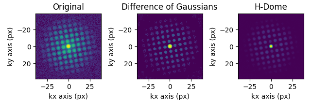
If your diffraction data is noisy, you might want to subtract the background from the dataset. Pyxem offers some built-in functionality for this, with the subtract_diffraction_background class method. Custom filtering is also possible, an example is shown in the ‘Filtering Data’-example.

import pyxem as pxm
import hyperspy.api as hs

s = pxm.data.tilt_boundary_data()

s_filtered = s.subtract_diffraction_background(
    "difference of gaussians",
    inplace=False,
    min_sigma=3,
    max_sigma=20,
)

s_filtered_h = s.subtract_diffraction_background("h-dome", inplace=False, h=0.7)


hs.plot.plot_images(
    [s.inav[2, 2], s_filtered.inav[2, 2], s_filtered_h.inav[2, 2]],
    label=["Original", "Difference of Gaussians", "H-Dome"],
    tight_layout=True,
    norm="symlog",
    cmap="viridis",
    colorbar=None,
)

  0%|          | 0/33 [00:00<?, ?it/s]
 24%|██▍       | 8/33 [00:00<00:00, 79.51it/s]
 48%|████▊     | 16/33 [00:00<00:00, 48.66it/s]
 67%|██████▋   | 22/33 [00:00<00:00, 36.63it/s]
 82%|████████▏ | 27/33 [00:00<00:00, 32.43it/s]
100%|██████████| 33/33 [00:00<00:00, 40.54it/s]
/home/docs/checkouts/readthedocs.org/user_builds/pyxem/envs/v0.21.0/lib/python3.11/site-packages/pyxem/utils/_background_subtraction.py:99: FutureWarning: `square` is deprecated since version 0.25 and will be removed in version 0.27. Use `skimage.morphology.footprint_rectangle` instead.
  regional_filter(frame / max_value, **kwargs), footprint=square(3)
/home/docs/checkouts/readthedocs.org/user_builds/pyxem/envs/v0.21.0/lib/python3.11/site-packages/hyperspy/misc/utils.py:1439: UserWarning: Possible precision loss converting image of type float32 to uint8 as required by rank filters. Convert manually using skimage.util.img_as_ubyte to silence this warning.
  output = function(test_data, **kwargs)

  0%|          | 0/33 [00:00<?, ?it/s]/home/docs/checkouts/readthedocs.org/user_builds/pyxem/envs/v0.21.0/lib/python3.11/site-packages/pyxem/utils/_background_subtraction.py:99: FutureWarning: `square` is deprecated since version 0.25 and will be removed in version 0.27. Use `skimage.morphology.footprint_rectangle` instead.
  regional_filter(frame / max_value, **kwargs), footprint=square(3)
/home/docs/checkouts/readthedocs.org/user_builds/pyxem/envs/v0.21.0/lib/python3.11/site-packages/hyperspy/misc/utils.py:1362: UserWarning: Possible precision loss converting image of type float32 to uint8 as required by rank filters. Convert manually using skimage.util.img_as_ubyte to silence this warning.
  output_array[islice] = function(data[islice], **kwargs)

  9%|▉         | 3/33 [00:00<00:01, 18.11it/s]
 21%|██        | 7/33 [00:00<00:01, 21.59it/s]
 33%|███▎      | 11/33 [00:00<00:01, 12.16it/s]
 39%|███▉      | 13/33 [00:00<00:01, 13.48it/s]
 45%|████▌     | 15/33 [00:01<00:01, 13.07it/s]
 52%|█████▏    | 17/33 [00:01<00:01, 13.31it/s]
 58%|█████▊    | 19/33 [00:01<00:01,  9.67it/s]
 64%|██████▎   | 21/33 [00:01<00:01, 10.64it/s]
 70%|██████▉   | 23/33 [00:01<00:00, 11.03it/s]
 76%|███████▌  | 25/33 [00:02<00:00, 10.97it/s]
 82%|████████▏ | 27/33 [00:02<00:00,  9.04it/s]
 88%|████████▊ | 29/33 [00:02<00:00,  9.58it/s]
 94%|█████████▍| 31/33 [00:02<00:00, 10.35it/s]
100%|██████████| 33/33 [00:02<00:00, 12.12it/s]

[<Axes: title={'center': 'Original'}, xlabel='kx axis (px)', ylabel='ky axis (px)'>, <Axes: title={'center': 'Difference of Gaussians'}, xlabel='kx axis (px)', ylabel='ky axis (px)'>, <Axes: title={'center': 'H-Dome'}, xlabel='kx axis (px)', ylabel='ky axis (px)'>]

Filtering Polar Images

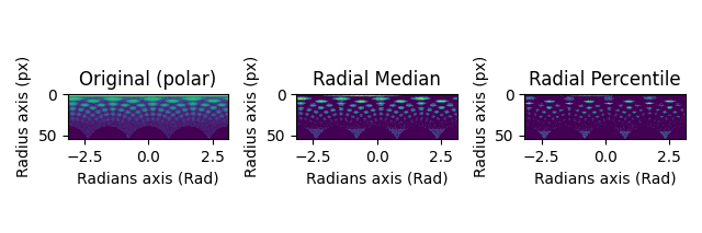
The available methods differ for Diffraction2D datasets and PolarDiffraction2D datasets.

Set the center of the diffraction pattern to its default, i.e. the middle of the image

s.calibration.center = None

Transform to polar coordinates

s_polar = s.get_azimuthal_integral2d(npt=100, mean=True)

s_polar_filtered = s_polar.subtract_diffraction_background(
    "radial median",
    inplace=False,
)

s_polar_filtered2 = s_polar.subtract_diffraction_background(
    "radial percentile",
    percentile=70,
    inplace=False,
)

hs.plot.plot_images(
    [s_polar.inav[2, 2], s_polar_filtered.inav[2, 2], s_polar_filtered2.inav[2, 2]],
    label=["Original (polar)", "Radial Median", "Radial Percentile"],
    tight_layout=True,
    norm="symlog",
    cmap="viridis",
    colorbar=None,
)

  0%|          | 0/17 [00:00<?, ?it/s]
  6%|▌         | 1/17 [00:03<00:55,  3.47s/it]
 47%|████▋     | 8/17 [00:03<00:02,  3.04it/s]
 82%|████████▏ | 14/17 [00:03<00:00,  6.05it/s]
100%|██████████| 17/17 [00:03<00:00,  4.54it/s]

  0%|          | 0/33 [00:00<?, ?it/s]
 70%|██████▉   | 23/33 [00:00<00:00, 224.95it/s]
100%|██████████| 33/33 [00:00<00:00, 233.67it/s]

  0%|          | 0/33 [00:00<?, ?it/s]
 33%|███▎      | 11/33 [00:00<00:00, 92.84it/s]
 64%|██████▎   | 21/33 [00:00<00:00, 77.38it/s]
 88%|████████▊ | 29/33 [00:00<00:00, 77.16it/s]
100%|██████████| 33/33 [00:00<00:00, 81.46it/s]

[<Axes: title={'center': 'Original (polar)'}, xlabel='Radians axis (Rad)', ylabel='Radius axis (px)'>, <Axes: title={'center': 'Radial Median'}, xlabel='Radians axis (Rad)', ylabel='Radius axis (px)'>, <Axes: title={'center': 'Radial Percentile'}, xlabel='Radians axis (Rad)', ylabel='Radius axis (px)'>]