Multi Phase Orientation Mapping

You can also calculate the orientation of the grains for multiple phases using the pyxem.signals.PolarSignal2D.get_orientation() method. This requires that you simulate the entire S2 space for the phase and then compare to the simulated diffraction.

For more information on the orientation mapping process see [CCAAnes+22]

import pyxem as pxm
from pyxem.data import fe_multi_phase_grains, fe_bcc_phase, fe_fcc_phase
from diffsims.generators.simulation_generator import SimulationGenerator
from orix.quaternion import Rotation
from orix.sampling import get_sample_reduced_fundamental

mulit_phase = fe_multi_phase_grains()

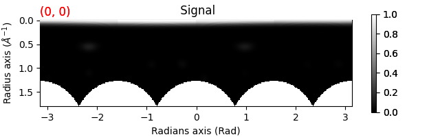
First we center the diffraction patterns and get a polar signal Increasing the number of npt_azim with give better polar sampling but will take longer to compute the orientation map The mean=True argument will return the mean pixel value in each bin rather than the sum this makes the high k values more visible

mulit_phase.calibration.center = None
polar_multi = mulit_phase.get_azimuthal_integral2d(
    npt=100, npt_azim=360, inplace=False, mean=True
)
polar_multi.plot()

• 
• 

[                                        ] | 0% Completed | 157.27 us
[                                        ] | 0% Completed | 100.47 ms
[                                        ] | 0% Completed | 200.87 ms
[                                        ] | 0% Completed | 301.26 ms
[                                        ] | 0% Completed | 401.65 ms
[                                        ] | 0% Completed | 502.05 ms
[                                        ] | 0% Completed | 602.44 ms
[                                        ] | 0% Completed | 702.83 ms
[                                        ] | 0% Completed | 803.83 ms
[                                        ] | 0% Completed | 904.23 ms
[                                        ] | 0% Completed | 1.00 s
[                                        ] | 0% Completed | 1.11 s
[                                        ] | 0% Completed | 1.21 s
[                                        ] | 0% Completed | 1.31 s
[                                        ] | 0% Completed | 1.41 s
[                                        ] | 0% Completed | 1.51 s
[                                        ] | 0% Completed | 1.61 s
[                                        ] | 0% Completed | 1.71 s
[                                        ] | 0% Completed | 1.81 s
[                                        ] | 0% Completed | 1.91 s
[                                        ] | 0% Completed | 2.01 s
[                                        ] | 0% Completed | 2.11 s
[                                        ] | 0% Completed | 2.21 s
[########################################] | 100% Completed | 2.31 s

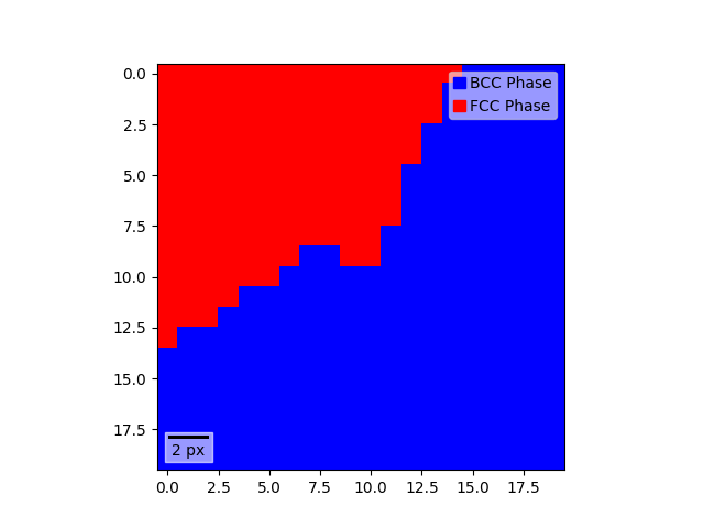
Now we can get make a simulation. In this case we want to set a minimum_intensity which removes the low intensity reflections. we also sample the S2 space using the :func`orix.sampling.get_sample_reduced_fundamental` We have two phases here so we can make a simulation object with both of the phases.

bcc = fe_bcc_phase()
fcc = fe_fcc_phase()
bcc.name = "BCC Phase"
fcc.name = "FCC Phase"
fcc.color = "red"
bcc.color = "blue"

generator = SimulationGenerator(200, minimum_intensity=0.05)
rotations_bcc = get_sample_reduced_fundamental(
    resolution=1, point_group=bcc.point_group
)
rotations_fcc = get_sample_reduced_fundamental(
    resolution=1, point_group=fcc.point_group
)

sim = generator.calculate_diffraction2d(
    [bcc, fcc],
    rotation=[rotations_bcc, rotations_fcc],
    max_excitation_error=0.1,
    reciprocal_radius=2,
    with_direct_beam=False,
)
polar_multi = polar_multi**0.5  # gamma correction
orientation_map = polar_multi.get_orientation(sim)


cmap = orientation_map.to_crystal_map()
cmap.plot()

[                                        ] | 0% Completed | 165.73 us
[                                        ] | 0% Completed | 100.48 ms
[                                        ] | 0% Completed | 200.84 ms
[                                        ] | 0% Completed | 304.90 ms
[                                        ] | 0% Completed | 405.39 ms
[                                        ] | 0% Completed | 505.71 ms
[                                        ] | 0% Completed | 606.06 ms
[                                        ] | 0% Completed | 706.42 ms
[                                        ] | 0% Completed | 810.33 ms
[                                        ] | 0% Completed | 912.71 ms
[                                        ] | 0% Completed | 1.01 s
[                                        ] | 0% Completed | 1.11 s
[                                        ] | 0% Completed | 1.21 s
[                                        ] | 0% Completed | 1.31 s
[                                        ] | 0% Completed | 1.41 s
[                                        ] | 0% Completed | 1.52 s
[                                        ] | 0% Completed | 1.62 s
[                                        ] | 0% Completed | 1.72 s
[                                        ] | 0% Completed | 1.82 s
[########################################] | 100% Completed | 1.92 s

[                                        ] | 0% Completed | 136.22 us
[########################################] | 100% Completed | 100.46 ms

[                                        ] | 0% Completed | 140.06 us
[########################################] | 100% Completed | 100.43 ms

[                                        ] | 0% Completed | 140.60 us
[########################################] | 100% Completed | 100.45 ms

sphinx_gallery_thumbnail_number = 3