Note
Go to the end to download the full example code.
Filtering Data#
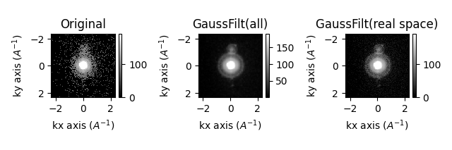
If you have a low number of counts in your data, you may want to filter the data to remove noise. This can be done using the filter function which applies some function to the entire dataset and returns a filtered dataset of the same shape.
from scipy.ndimage import gaussian_filter
from dask_image.ndfilters import gaussian_filter as dask_gaussian_filter
import pyxem as pxm
import hyperspy.api as hs
import numpy as np

s = pxm.data.mgo_nanocrystals(allow_download=True)  # MgO nanocrystals dataset

s_filtered = s.filter(
    gaussian_filter, sigma=1.0, inplace=False
)  # Gaussian filter with sigma=1.0

s_filtered2 = s.filter(
    gaussian_filter, sigma=(1.0, 1.0, 0, 0), inplace=False
)  # Only filter in real space

hs.plot.plot_images(
    [s.inav[10, 10], s_filtered.inav[10, 10], s_filtered2.inav[10, 10]],
    label=["Original", "GaussFilt(all)", "GaussFilt(real space)"],
    tight_layout=True,
    vmax="99th",
)
  0%|                                               | 0.00/104M [00:00<?, ?B/s]
  0%|                                       | 17.4k/104M [00:00<10:24, 167kB/s]
  0%|                                       | 54.3k/104M [00:00<06:15, 278kB/s]
  0%|                                        | 129k/104M [00:00<03:37, 480kB/s]
  0%|                                        | 275k/104M [00:00<02:02, 848kB/s]
  1%|▏                                      | 567k/104M [00:00<01:06, 1.56MB/s]
  1%|▍                                     | 1.17M/104M [00:00<00:34, 3.01MB/s]
  2%|▊                                     | 2.38M/104M [00:00<00:17, 5.83MB/s]
  4%|█▍                                    | 3.95M/104M [00:00<00:11, 8.79MB/s]
  5%|██                                    | 5.54M/104M [00:00<00:09, 10.8MB/s]
  7%|██▌                                   | 7.16M/104M [00:01<00:07, 12.3MB/s]
  8%|███▏                                  | 8.78M/104M [00:01<00:07, 13.3MB/s]
 10%|███▊                                  | 10.4M/104M [00:01<00:06, 14.0MB/s]
 12%|████▍                                 | 12.0M/104M [00:01<00:06, 14.5MB/s]
 13%|████▉                                 | 13.7M/104M [00:01<00:06, 14.9MB/s]
 15%|█████▌                                | 15.4M/104M [00:01<00:05, 15.2MB/s]
 16%|██████▏                               | 17.1M/104M [00:01<00:05, 15.6MB/s]
 18%|██████▊                               | 18.8M/104M [00:01<00:05, 15.9MB/s]
 20%|███████▍                              | 20.6M/104M [00:01<00:05, 16.2MB/s]
 21%|████████▏                             | 22.4M/104M [00:01<00:04, 16.6MB/s]
 23%|████████▊                             | 24.2M/104M [00:02<00:04, 16.8MB/s]
 25%|█████████▍                            | 26.0M/104M [00:02<00:04, 17.1MB/s]
 27%|██████████▏                           | 27.9M/104M [00:02<00:04, 17.3MB/s]
 28%|██████████▊                           | 29.7M/104M [00:02<00:04, 17.4MB/s]
 30%|███████████▌                          | 31.6M/104M [00:02<00:04, 17.6MB/s]
 32%|████████████▏                         | 33.4M/104M [00:02<00:03, 17.8MB/s]
 34%|████████████▉                         | 35.4M/104M [00:02<00:03, 18.3MB/s]
 36%|█████████████▌                        | 37.2M/104M [00:02<00:03, 18.2MB/s]
 38%|██████████████▎                       | 39.2M/104M [00:02<00:03, 18.6MB/s]
 40%|███████████████                       | 41.3M/104M [00:03<00:03, 18.9MB/s]
 42%|███████████████▊                      | 43.3M/104M [00:03<00:03, 19.2MB/s]
 44%|████████████████▌                     | 45.4M/104M [00:03<00:03, 19.5MB/s]
 46%|█████████████████▎                    | 47.6M/104M [00:03<00:02, 19.9MB/s]
 48%|██████████████████                    | 49.7M/104M [00:03<00:02, 20.1MB/s]
 50%|██████████████████▉                   | 51.9M/104M [00:03<00:02, 20.3MB/s]
 52%|███████████████████▋                  | 54.0M/104M [00:03<00:02, 20.4MB/s]
 54%|████████████████████▍                 | 56.2M/104M [00:03<00:02, 20.7MB/s]
 56%|█████████████████████▎                | 58.4M/104M [00:03<00:02, 20.9MB/s]
 58%|██████████████████████                | 60.7M/104M [00:03<00:02, 21.2MB/s]
 60%|██████████████████████▉               | 63.0M/104M [00:04<00:01, 21.4MB/s]
 63%|███████████████████████▊              | 65.3M/104M [00:04<00:01, 21.6MB/s]
 65%|████████████████████████▌             | 67.6M/104M [00:04<00:01, 21.7MB/s]
 67%|█████████████████████████▍            | 69.9M/104M [00:04<00:01, 21.9MB/s]
 69%|██████████████████████████▎           | 72.2M/104M [00:04<00:01, 22.0MB/s]
 71%|███████████████████████████▏          | 74.5M/104M [00:04<00:01, 22.1MB/s]
 74%|████████████████████████████          | 76.9M/104M [00:04<00:01, 22.5MB/s]
 76%|████████████████████████████▉         | 79.3M/104M [00:04<00:01, 22.7MB/s]
 78%|█████████████████████████████▊        | 81.8M/104M [00:04<00:00, 23.0MB/s]
 81%|██████████████████████████████▋       | 84.3M/104M [00:04<00:00, 23.3MB/s]
 83%|███████████████████████████████▋      | 86.8M/104M [00:05<00:00, 23.9MB/s]
 86%|████████████████████████████████▌     | 89.2M/104M [00:05<00:00, 23.9MB/s]
 88%|█████████████████████████████████▍    | 91.8M/104M [00:05<00:00, 24.0MB/s]
 90%|██████████████████████████████████▍   | 94.4M/104M [00:05<00:00, 24.4MB/s]
 93%|███████████████████████████████████▎  | 96.9M/104M [00:05<00:00, 24.4MB/s]
 95%|████████████████████████████████████▎ | 99.6M/104M [00:05<00:00, 24.8MB/s]
 98%|██████████████████████████████████████▏| 102M/104M [00:05<00:00, 25.0MB/s]
  0%|                                               | 0.00/104M [00:00<?, ?B/s]
100%|████████████████████████████████████████| 104M/104M [00:00<00:00, 412GB/s]

[<Axes: title={'center': 'Original'}, xlabel='kx axis ($A^{-1}$)', ylabel='ky axis ($A^{-1}$)'>, <Axes: title={'center': 'GaussFilt(all)'}, xlabel='kx axis ($A^{-1}$)', ylabel='ky axis ($A^{-1}$)'>, <Axes: title={'center': 'GaussFilt(real space)'}, xlabel='kx axis ($A^{-1}$)', ylabel='ky axis ($A^{-1}$)'>]
"""
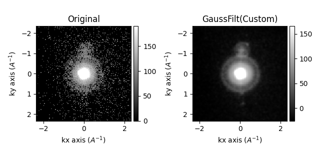
The `filter` function can also be used with a custom function as long as the function
takes a numpy array as input and returns a numpy array of the same shape.
"""
def custom_filter(array):
filtered = gaussian_filter(array, sigma=1.0)
return filtered - np.mean(filtered)
s_filtered3 = s.filter(custom_filter, inplace=False) # Custom filter
hs.plot.plot_images(
[s.inav[10, 10], s_filtered3.inav[10, 10]],
label=["Original", "GaussFilt(Custom)"],
tight_layout=True,
vmax="99th",
)
[<Axes: title={'center': 'Original'}, xlabel='kx axis ($A^{-1}$)', ylabel='ky axis ($A^{-1}$)'>, <Axes: title={'center': 'GaussFilt(Custom)'}, xlabel='kx axis ($A^{-1}$)', ylabel='ky axis ($A^{-1}$)'>]
"""
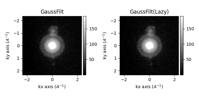
For lazy datasets, functions which operate on dask arrays can be used. For example,
the `gaussian_filter` function from `scipy.ndimage` is replaced with the `dask_image`
version which operates on dask arrays.
"""
s = s.as_lazy() # Convert to lazy dataset
s_filtered4 = s.filter(
dask_gaussian_filter, sigma=1.0, inplace=False
) # Gaussian filter with sigma=1.0
hs.plot.plot_images(
[s_filtered.inav[10, 10], s_filtered4.inav[10, 10]],
label=["GaussFilt", "GaussFilt(Lazy)"],
tight_layout=True,
vmax="99th",
)
[<Axes: title={'center': 'GaussFilt'}, xlabel='kx axis ($A^{-1}$)', ylabel='ky axis ($A^{-1}$)'>, <Axes: title={'center': 'GaussFilt(Lazy)'}, xlabel='kx axis ($A^{-1}$)', ylabel='ky axis ($A^{-1}$)'>]
Total running time of the script: (0 minutes 30.507 seconds)